 Volume
2, Number 1, 2015, 67–93 journal homepage:
region.ersa.org
Volume
2, Number 1, 2015, 67–93 journal homepage:
region.ersa.orgForecasting employment location choices by Discrete Choice Models: A sensitivity analysis to scale and implications for LUTI models
1 Université Catholique de Louvain, Louvain-la-Neuve, Belgium (email: jonathan.jones@uclouvain.be)2 Université Catholique de Louvain, Louvain-la-Neuve, Belgium (email: isabelle.thomas@uclouvain.be)
3 Université Catholique de Louvain, Louvain-la-Neuve, Belgium (email: dominique.peeters@uclouvain.be) Received: 6 November 2014/Accepted: 21 May 2015
Abstract. This paper proposes an empirical analysis of the sensitivity of Discrete Choice Model (DCM) to the size of the spatial units used as choice set. This is related to the well-documented Modifiable Areal Unit Problem). Employment location choices in Brussels, Belgium are used for the case study. DCMs are implemented within different Land Use and Transport Interactions (LUTI) models (UrbanSim, ILUTE) to forecast jobs and household location choices. Nevertheless, no studies have yet assessed their sensitivity to the size of the Basic Spatial Units (BSU) in an urban context. The results show significant differences in parameter estimates between BSU level. Under the assumption from the LUTI model that new jobs are distributed among the study area proportionally to the utility level predicted by the DCM for each BSU level, it is demonstrated that the spatial distribution of these new jobs varies with the size of the BSUs. These findings indicate that the BSU level used in the model can influence the output of a LUTI model relying on DCM to forecast location choices of agents and, therefore, have important operational implications for land-use planning.
JEL classification: C25, R30
Key words: Discrete Choice Models, Scale, Brussels
1 Introduction
Discrete Choice Models (DCM) have been widely used to forecast location choices for economic activities (see Arauzo-Carod et al. 2010). Like other econometric methods, they may however be influenced by spatial biases when the choice set consists in areal units (see Section 2). For instance, Arauzo-Carod, Manjón-Antolín (2004), by comparing firm’s location choices in Catalonia (Spain) for three levels of administrative units, found significant differences in the parameter estimates of the DCM. This issue is particularly relevant for Land-Use and Transport Interactions (LUTI) models, since most state-of-the-art LUTI models rely on DCMs to forecast agents’ location choices (e.g. CUF-2, see Landis, Zhang 1998a, Landis, Zhang 1998b; UrbanSim, see Waddell 2000, Noth et al. 2003; or ILUTE, see Salvini, Miller 2005, Hunt et al. 2005; see Wegener 2004 for review). Moreover, the availability of detailed data sets on firms’ locations means that empirical studies have evolved from aggregated to disaggregated areas (e.g. census wards instead of municipalities or regions; see McCann, Sheppard 2003, Guimaraes et al. 2004, and Arauzo-Carod et al. 2010). A similar trend from large to small Basic Spatial Units (BSU) can be observed in LUTI models.
Discrete Choice Models allow for the computing of the utility of each areal unit in the choice set and thus the probability that an agent selects a given BSU. This framework is consistent with the analysis of employment location choices, because the utility theory relies directly on location selection by profit maximizing firms (Shukla, Waddell 1991). However, the sensitivity of DCM to the size (equivalent to the number) of the BSUs used as a choice set remains largely an open question. In particular, existing works (Arauzo-Carod, Manjón-Antolín 2004) are based on areal units larger than those generally used in LUTI models, which utilize either municipalities or census tracts. De Palma et al. (2007) estimated household location choices in Paris from two levels of small urban areas and found variations in the parameter estimates, but do not provide a systematic comparison of these variations.
The general aim of this paper is thus to examine how, in an urban context, DCM are influenced by a change of the size of the BSUs used as the choice set. To provide an answer as complete as possible to this question, we consider three successive research questions.
First, do the parameter estimates of DCM vary with the size of the spatial units that constitute the choice set? An empirical analysis of employment location choice is conducted for two spatial patterns: monocentric, using jobs in services, and polycentric, using industrial activities (see Section 3). The case study is the urban region of Brussels (Belgium), and four levels of hierarchical administrative units are used as the BSUs. Let us add here that the aim of the paper is not to study industrial location choices. The data set was used because of its availability, and the two activities sectors serve as proxies for the different spatial pattern. The econometric framework is identical to the DCM implemented in the UrbanSim LUTI model: a linear-in-parameter, utility maximizing, multinomial logit model (MNL) (see Waddell et al. 2003).
Second, are the variations of parameter estimates between BSU levels significant compared to misspecification issues? Amrhein (1995) and Briant et al. (2010), among others, show that the latter may be larger than the former. Hence five different specifications are estimated for each location choice model to allow for a comparison of variations between BSU levels and specifications and, therefore, of the relative importance of spatial biases versus misspecification issues.
Third, what are the operational implications? A clustering procedure is conducted to compare the structure of the probability of location through scales. Furthermore, assuming that new jobs are created and are allocated through the BSUs proportionally to the predicted utility level, as in a LUTI model, we test for variation in the locational distribution of these new jobs per spatial units when simulated for different BSUs.
To cover these questions, the paper is organized as follows: Challenges arising from the use of spatial choice set in a DCM are shortly presented in Section 2. The case studies and the methodology are detailed in Section 3. Section 4 presents the results, which are then discussed in Section 5. And lastly, the conclusion is presented in Section 6.
2 Methodological challenges of DCM with spatial choice set
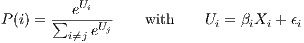
Compared to the classical stated preferences framework, the implementation of DCM in LUTI models rely on revealed preferences data sets (i.e. data sets with the actual location of the firms; see Wardman 1988 for a comparison of these approaches). The reason for this is that LUTI models do not use a continuous representation of space. The choice set corresponds to areal units, such as census tracts or municipalities, and includes a very large number of alternatives. Fundamentals of DCM are simple: an agent selects one alternative among those available (the choice set), in order to maximize his utility at the time when the choice is made (Ben Akiva, Lerman 1985). These alternatives have to be mutually exclusive, exhaustive and their number must be finite (Train 2003) conditions that all hold for areal units. In the classical specification of an MNL model, the probability that an alternative i is selected (P(i), see Equation 1) depends on its utility Ui, which itself relies on Xi, the characteristics of i.
 | (1) |
For computational tractability purposes, DCM implemented in LUTI models rely thus on the classical linear-in-parameter, utility maximization (MNL model with random sampling of alternatives (Waddell 2002, Hunt et al. 2005, see also Section 3). This traditional MNL model suffers criticisms on both theoretical and operational points of view when applied on a spatial choice set.
One common problem for a choice set composed of areal units is that the Independence of Irrelevant Alternatives assumption is unlikely to hold in the presence of spatial autocorrelation among alternatives (Sener et al. 2011). This bias can be controlled by accounting for shared unobserved characteristics between adjacent alternatives (Generalized Spatially Correlated Logit, see Guo, Bhat 2004, Sener et al. 2011), or by including a spatially weighted average to the utility function of each alternative (Alamá-Sabater et al. 2011). None of these models are, however, implemented in operational LUTI models (see Wegener 2004). The use of nested logit has also been suggested (see Cornelis et al. 2012 for an application to residential location choice in Belgium). Such a framework was also implemented in different LUTI models (IRPUD, see Wegener 2011, UrbanSim, see Waddell et al. 2003, and PECAS, see Hunt et al. 2009). However, the different levels rarely consist of spatial units (such as the urban areas/suburbs/commuting zone/rural areas typology used by Cornelis et al. 2012), but rather of different types of buildings (e.g. houses, flats, etc.).
The choice set can also be different among agents (Thill 1992), especially for residential location choices (see Pagliara, Wilson 2010, for review). The random sampling of alternatives assumes a perfect knowledge of all alternatives, which is unrealistic given the limited capacity of agents for gathering information (see Fotheringham et al. 2000, Meester, Pellenberg 2006). Imperfect information is captured in some LUTI models (e.g. IRPUD, see Wegener 2011), but they constitute the exceptions.
The sensitivity to the size of the areal units used in the choice set of the DCM (i.e. the scale effect component of the Modifiable Areal Unit Problem [MAUP], see Openshaw, Taylor 1979), which is the scope of this paper, has been far less studied than other econometric methods. Arauzo-Carod, Manjón-Antolín (2004) compared firm’s location choices for three levels of administrative units, using both DCM and Count Data Models (CDM). They observe significant differences between parameter estimates and conclude that location choice factors do not act uniformly with the scale over broad geographic regions. However, their study area (Catalonia region, Spain) and areal units (provinces or municipalities) cannot be compared easily to typical applications of LUTI models (metropolitan areas with smaller BSUs such as census tract). Hence, there is a need to extend the sensitivity analysis to an urban case study. An example for residential location choice in Paris (France) can be found in de Palma et al. (2007): they conclude that the factors driving these choices vary with the size of the spatial unit considered (municipalities or grid cells of 500 by 500 meters), but they do not provide a complete analysis on the influence of the MAUP. Note that for smaller BSUs, another difficulty comes from the fact that the relevant extension of the neighbourhood taken into account by agents can exceed the size of these areal units. Improvements of the classical MNL specification, such as a multi-scale modelling structure, should then be used (Guo, Bhat 2004). But this specification is itself sensitive to the definition of the neighbourhood (Guo, Bhat 2007), and currently not implemented in LUTI models.
Finally, an ideal specification of DCM with spatial choice set is one that is independent of the level of aggregation in the definition of the zone. That is to say, a model where the probability of a zone i, created by merging two zones j and k, is equal to the sum of the probabilities of j and k, such that P(i) = P(j) + P(k). However, that equality only holds if the utilities need to be expressed logarithmically, but such a specification is far more computationally intensive than the classical linear-in-parameters specification, and not commonly implemented in econometric software (Train 2003). This example does not correspond exactly to the situation assessed in this work, since the estimation of DCM for two different level of BSU will lead to two independent set of parameter estimates. However, it illustrates that the linear-in-parameter MNL model is far from ideal for spatial choice sets.
3 Methods and data
3.1 Case studies
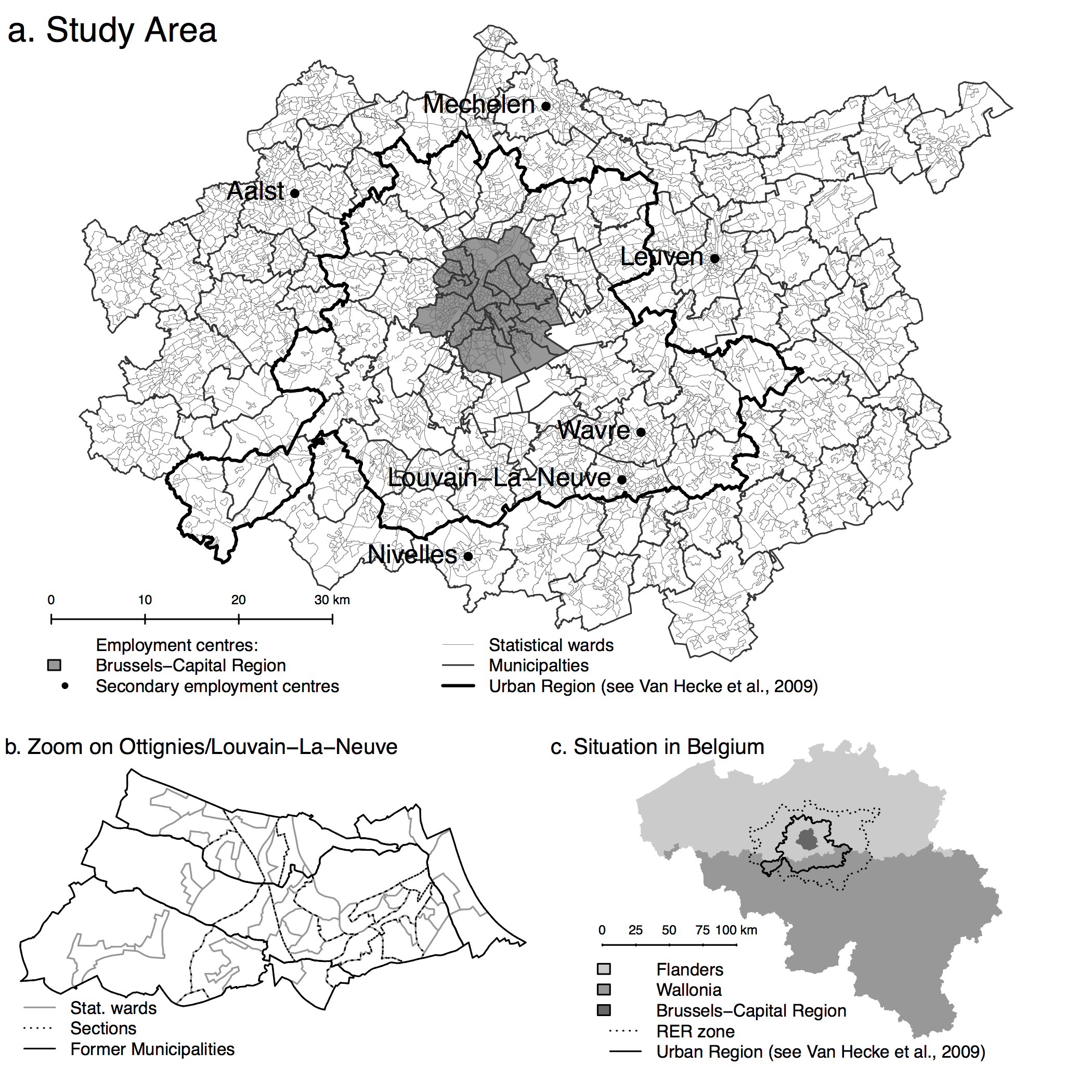
The study area is centred on the city of Brussels, Belgium – the main employment center of the country. Its administrative delineation, the Brussels-Capital Region (BCR), included 650,000 jobs and 19% of the GDP in 2007 (Thisse, Thomas 2007, 2010). As in many other cities, due to urban sprawl, this official delineation of Brussels does not correspond anymore to the city’s area of influence (Dujardin et al. 2007, Cheshire 2010), and thus functional delineations should be used.
The use of a real-world application was driven mostly by data availability. Administrative and statistical delineations in Belgium have a high level of spatial detail (see below), thus allowing us to study the effect of scale in a more continuous way than in previous works. The influence of the MAUP on econometric estimations often relies on synthetic data sets (see Fotheringham, Wong 1991; for correlation and linear regression, see Amrhein 1995), but no comparable works exist for DCM. In particular, Arauzo-Carod, Manjón-Antolín (2004) and de Palma et al. (2007) both rely on empirical case studies. Synthetic data sets remove the potential misspecification bias, since they allow controlling the relationship between dependant and independent variables. They also have the advantage of permitting more systematic variations of the size of the BSU level. However, we believe that sensitivity analysis based on empirical data provides more direct insights for operational applications of DCM, hence the use of Brussels.
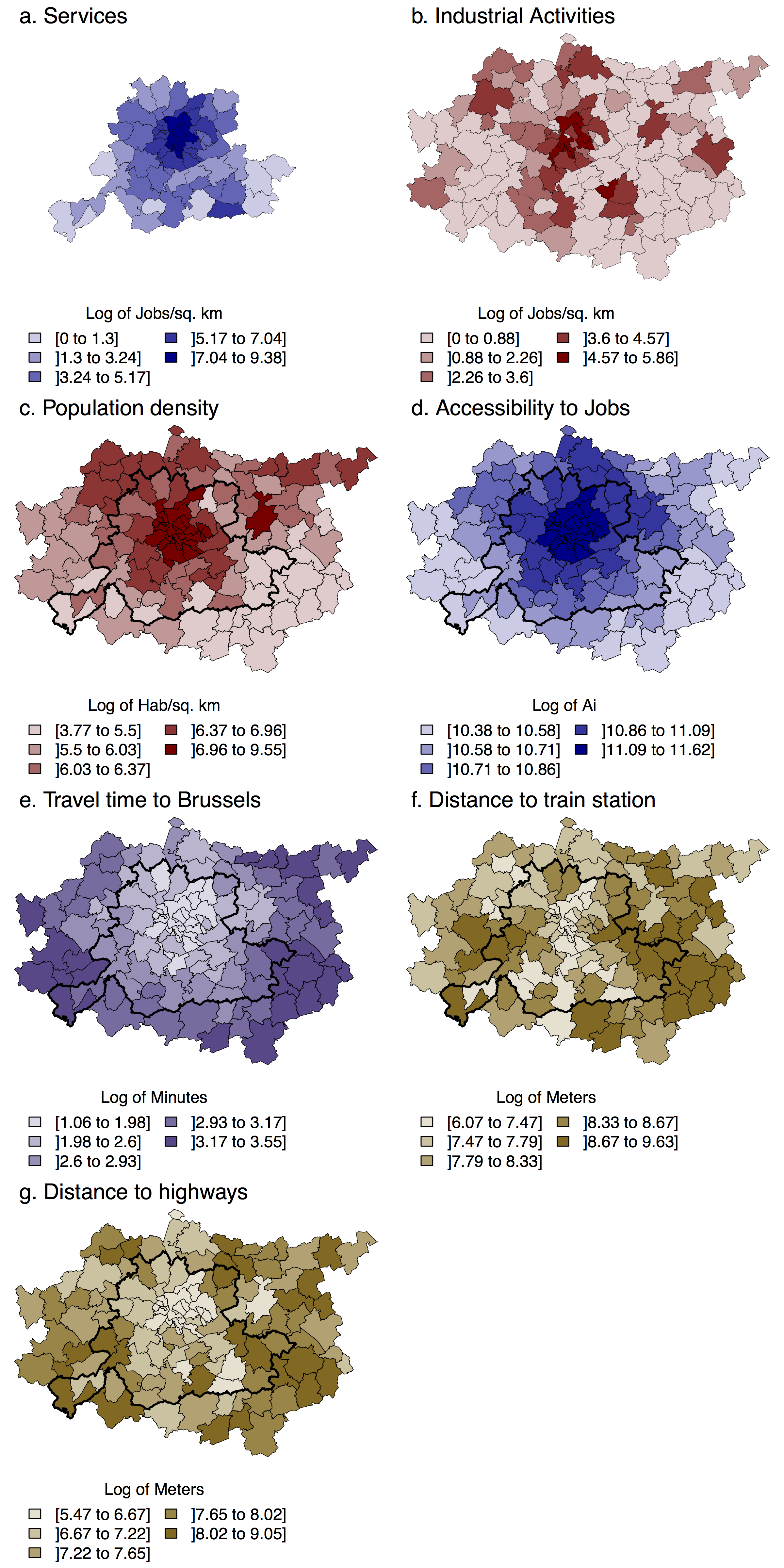
Moreover, we can expect that the sensitivity of DCM to scales will be affected by the underlying spatial distribution of firms, and thus employment: if jobs are concentrated in a large employment center, this center will always emerge from the neighbouring areas. On the contrary, if jobs are scattered through small employment centres, these small centres may be diluted within their neighbourhood for larger BSUs. To assess this potential effect, two case studies are considered, corresponding to two different spatial patterns. The first case study (Monocentric) examines the location choices of jobs in the tertiary sector on a small and monocentric study area, the Urban Region of Brussels. Defined by (van Hecke et al. 2009), this region corresponds to the area with strong direct links to the CBD of Brussels, notably through commuting. The combination of the high centrality of jobs in tertiary activities and of a small study area results in a monocentric case, with most of the job concentrated in the CBD of Brussels (Figure 1a).
In the second case study (Polycentric) location choices of industrial jobs are estimated on a large, polycentric study area. The so-called RER (for “Réseau Express Régional”) zone (Moniteur Belge 2004) has been used. It corresponds to the extension of a fast train network to and from Brussels, which is currently under construction, and includes different secondary cities: Aalst, Mechelen and Leuven in the north (Flanders) and Wavre and Louvain-La-Neuve in the south (Wallonia). Together with the less concentrated distribution of jobs observed for industrial activities than for services, the larger extent of this area under study leads to a more polycentric structure (Figure 1b). Figure A.1 (in Appendix) shows the extension of these studies areas, and the administrative units used as BSUs (see also Table 1).
3.1.1 Basic spatial units
Four levels of administrative and statistical units are used in the analyses, the higher of which is the municipality. Each can be subdivided into former municipalities. Moreover, for census purposes, former municipalities can be divided into sections, themselves composed of several statistical wards. These statistical wards are the smallest areal unit for which data are available from the Belgian Directorate General Statistics and Economical Information Office (DGSIE 2013) are the statistical wards. Note that they are supposed to be homogeneous on social, functional or morphological (land-use) point of view (van Hecke et al. 2009). These BSU level are hierarchical, meaning that a BSU of level n is strictly contained in only one BSU of level n+1 (see Figure A.1b, in Appendix)1 . Conversely, it means that statistical wards can be aggregated recursively into sections, former municipalities, and municipalities, with a perfect overlap of their boundaries. Since this paper focuses on operational implications, we do not consider artificial territorial units (i.e. division of space based on raster, gridcells, or Thiessen polygons).
| Monocentric | Polycentric | ||||||||
| Basic Spatial Units | n | Min | Mean | Max | n | Min | Mean | Max | |
| Statistical wards | 2074 | 0.01 | 0.7 | 14.9 | 4223 | 0.01 | 0.9 | 15.9 | |
| Sections | 550 | 0.01 | 2.6 | 15.4 | 1217 | 0.01 | 3.3 | 16.5 | |
| Former municipalities | 173 | 0.25 | 8.7 | 45 | 473 | 0.25 | 8.7 | 45 | |
| Municipalities | 62 | 1.06 | 23.8 | 68.6 | 126 | 1.06 | 32.4 | 96.4 | |
Few studies exist on location choices of firms or jobs for our case study, except Baudewyns (1999) and Baudewyns et al. (2000) who use a different framework (stated preferences). Nevertheless, Marissal et al. (2006) show that jobs remain concentrated in central places (see also Riguelle et al. 2007) even if between 1991 and 2001 job growth was systematically lower in the city center than in the suburbs. The tertiary sector (i.e. the Monocentric case study and financial activities in particular) is highly concentrated in the Brussels-Capital Region, while non-trade services are less concentrated but still reflect the distribution of the population and, consequently, the urban structure (Marissal et al. 2006). Secondary cities are of a higher importance for industrial activities (i.e. the Polycentric case study), especially in Flanders.
3.1.2 Employment location
For job location data, the Home-To-Work Travel (HTWT) Survey of 2008 (see Witlox et al. 2011, van Malderen et al. 2012) was used. This survey is a legal requirement, which allows a response rate above 90%. For all firms located in Belgium with at least one hundred employees, the survey gives the geographic coordinates of all plants of more than thirty employees. The NACE-BEL 2008 2-digits classification of economic activities (DGSIE 2013) was used to select the firms in industrial activities (NACE code from 12 to 45 included) that compose the Polycentric case study, and in services (NACE codes higher than 45), for the Monocentric case study. Note that since the HTWT data set is limited to firms of more than one hundred employees, it only accounts for 57% of the total number of jobs in tertiary sector and 43% for industrial activities (ONSS 2015). It should also be noted that the HTWT database includes all jobs at one given time, rather than jobs that recently relocated. Figure 1 shows the spatial distribution of jobs for the two case studies considered in this paper. Descriptive statistics of the number of jobs per BSU are given by Table 1.
3.1.3 Zonal characteristics
The econometric model used in this work (see Section 3.2) follows the neoclassical perspective (Hayter 1997), which assumes that agents are rational and have perfect information (see Shukla, Waddell 1991, Waddell et al. 2003). In such a conceptual framework, location determinants are cost-driving factors (e.g. agglomeration economies, transport infrastructure, and technology or human capital; see Arauzo-Carod et al. 2010 for review). The variables used in this work attempt to cover these three categories. There are two reasons why we chose such variables instead of the wide range of variables that could be taken as a proxy. First, given the large variations in the size of the BSU level (see Table 1), we restrained ourselves to variables expected to play a role at all scales, excluding local characteristics that could have been significant for smaller BSUs alone (see de Palma et al. 2007). Furthermore, only relatively simple variables were considered: Variables that were directly available (see below) or do not require complex GIS data processing and could be aggregated into larger BSUs by sums or means.
For agglomeration economies, the density of jobs was selected. However, since a one time-step data set was used (and not firms that recently relocated), explaining the employment location by the employment density lead to a major endogeneity concern. Preliminary analysis proved that including the employment density in the model precluded any other variables to have a significant effect, and this variable has thus been excluded. Another problem is encountered for technology and human capital that mostly rely on socio-economic factors: The Directorate General Statistics and Economic Information (DGSIE) only disclose real estate prices at the municipalities level. Most studies on real estate prices in Belgium (Goffette-Nagot et al. 2011, Cavailhès, Thomas 2012, Jones et al. 2015) thus use municipalities as the level of analysis. There is no example of the estimation of a disaggregated indicator of real estate values at the statistical ward level (which would be a complete work in itself).
Moreover, simply attributing to all lower-level BSU the value of the municipality to which it belongs may bias econometric estimations and do not seem a good option in a work dedicated to the sensitivity of econometric estimations to scale. Hence, real estate prices will not be used in this work. Population density (POP_DENS), available from the DGSIE at the statistical ward level, is instead used as a proxy. It is defined as the number of inhabitants per square kilometre. Population density is likely to have a positive influence on utilities for larger BSUs (municipalities and former municipalities) since it will represent, at this scale, urban areas. However, for smaller BSUs, a negative influence can be assumed due to competition for land (a high population density meaning that there is no or few spaces left for other activities).
Transport and accessibility amenities are represented by four variables: travel time (TIME_BXL) to Brussels by car (in minutes), with congestion included, is used as an indicator for accessibility to the main employment center. Travel times are computed between the centroid of each of the BSUs and the centroid of the municipality of Brussels (data from Vandenbulcke et al. 2007). The accessibility to jobs (ACC_JOBS) is a Shimbel index of the travel time by car (data from Vandenbulcke et al. 2007) between i and all other spatial units of the same level in Belgium, weighted by the total number of jobs (self-employed excluded) located in these BSUs, from the HTWT database. Local amenities are accounted for by the Euclidean distance between the centroid of each of the BSU and (a) the closest IC/IR trains station2 (DIST_TRAIN) and (b) the closest entry/exit on a highway (DIST_HGW). In Belgium, Baudewyns et al. (2000) found a positive impact of transport infrastructure on location choice of firms and similar findings are numerous in the empirical literature (see Arauzo-Carod et al. 2010 for review). These variables are thus expected to have a positive parameter estimate for both case studies and for all BSU level.
Figure 1 shows the distribution of these explanatory factors and their descriptive statistics are given by Table 2. For BSU level larger than the statistical ward, the databases were generated by aggregation of the initial data either by sums or means. Note that in the econometric model, all of these variables are expressed logarithmically.
3.2 Econometric estimations and sensitivity analysis
3.2.1 Location choice model
Our framework is identical to the Employment Location Choice Model in UrbanSim (see Waddell et al. 2003). It corresponds to the classical linear-in-parameters, utility maximizing MNL model (Ben Akiva, Lerman 1985). No alternative specific constants are included. As proposed by McFadden (1978), rather than using the complete choice set we select for each observation a subset composed of the selected alternative and nine randomly selected non-chosen alternatives. The model is based on an individual representation of jobs (rather than firms). Hence, no firm-specific factors are included and the only characteristics of the jobs taken into account are their current location. Explanatory variables are thus limited to site-specific factors. This choice matches those made in recent applications of the UrbanSim model, where the characteristics of the firm are not taken into account (see e.g. Waddel et al. 2007, Nicolas et al. 2008, Cabrita et al. 2015 for Brussels).
It is however clear that the little effort made to jointly consider plant and zone factors remains one weakness of DCM, and consequently of our work (Arauzo-Carod et al. 2010; see Arauzo-Carod, Manjón-Antolín 2004 for an analysis that considers both the size of the firms and of the areal units). Models for Monocentric and Polycentric case studies are estimated independently, the dependent variable being in both cases the type of BSU where the job is located. Estimations are performed in R, with the ’mlogit’ package (Croissant 2012).
3.2.2 Sensitivity analysis
For each case study, the methodology was the following. Six different combinations of the independent variables were drawn (Table 3). They focus on socio-economic characteristics, on accessibility indicators or on a mix of these factors. Two reasons explain the use of estimation of different specifications. First, Amrhein (1995) and Briant et al. (2010) argue that for econometric models, the misspecification’s issue induces larger variations of parameter estimates than those observed between BSU level. It was thus necessary to test this issue here (which corresponds to our second research question). Moreover, no studies on employment location choices based on a DCM model exist for our case study (see Section 3.1).
| BSU | Variables | Min | Mean | Max | SD
|
| Statistical | Log(POP_DENS) | 0 | 6.33 | 10.71 | 2.24 |
| wards | Log(ACC_JOBS) | 10.68 | 10.82 | 11.67 | 0.30 |
| Log(TIME_BXL) | 0 | 2.68 | 3.8 | 0.81 | |
| Log(DIST_TRAIN) | 4.5 | 8.02 | 9.75 | 0.82 | |
| Log(DIST_HGW) | 3.57 | 7.34 | 9.49 | 0.98 | |
| Jobs in Services | 0 | 164 | 10 620 | 679 | |
| Jobs in Industry | 0 | 15 | 3 281 | 126 | |
| Sections | Log(POP_DENS) | 0 | 5.99 | 10.34 | 1.59 |
| Log(ACC_JOBS) | 10.28 | 10.77 | 11.64 | 0.28 | |
| Log(TIME_BXL) | 0 | 2.78 | 3.8 | 0.66 | |
| Log(DIST_TRAIN) | 5.47 | 8.15 | 9.74 | 0.78 | |
| Log(DIST_HGW) | 4.4 | 7.5 | 9.48 | 0.94 | |
| Jobs in Services | 0 | 621 | 24 238 | 1 887 | |
| Jobs in Industry | 0 | 54 | 3 281 | 250 | |
| Former | Log(POP_DENS) | 0 | 5.71 | 9.55 | 1.23 |
| municipalities | Log(ACC_JOBS) | 10.28 | 10.70 | 11.62 | 0.24 |
| Log(TIME_BXL) | 0 | 2.92 | 3.8 | 0.54 | |
| Log(DIST_TRAIN) | 6.07 | 8.32 | 9.74 | 0.71 | |
| Log(DIST_HGW) | 5.21 | 7.72 | 9.48 | 0.83 | |
| Jobs in Services | 0 | 1 976 | 58 618 | 5 481 | |
| Jobs in Industry | 0 | 139 | 4 796 | 461 | |
| Municipalities | Log(POP_DENS) | 3.77 | 6.24 | 9.55 | 1.06 |
| Log(ACC_JOBS) | 10.31 | 10.80 | 11.62 | 0.28 | |
| Log(TIME_BXL) | 0 | 2.71 | 3.73 | 0.57 | |
| Log(DIST_TRAIN) | 6.07 | 8.1 | 9.62 | 0.68 | |
| Log(DIST_HGW) | 5.47 | 7.45 | 9.3 | 0.81 | |
| Jobs in Services | 0 | 5 514 | 103 675 | 13 628 | |
| Jobs in Industry | 0 | 522 | 6 282 | 1 033 | |
| Specifications | ||||||
| Variables | (1) | (2) | (3) | (4) | (5) | |
| POP_DENS | 0 | 1 | 0 | 1 | 0 | |
| ACC_JOBS | 1 | 1 | 0 | 0 | 1 | |
| TIME_BXL | 0 | 0 | 1 | 1 | 1 | |
| DIST_TRAIN | 1 | 1 | 1 | 1 | 1 | |
| DIST_HGW | 1 | 1 | 1 | 1 | 1 | |
We would stress here that our goal is not to find the best explanatory model for employment location choices in Brussels. This data set was used because it was available and it allows for comparing different spatial patterns (monocentric and polycentric). Hence, only simple variables are used as independent factors. One could wonder if the use of a more detailed model will not reduce variations across scales. This is, however, not our opinion, since previous work using more complex specifications found significant variations of parameter estimates between BSU level (Arauzo-Carod, Manjón-Antolín 2004, de Palma et al. 2007). The use of a more advanced method is perhaps a better way, with the restriction that they are not, to the exception of nested logit, implemented in LUTI models, nor in most operational applications of DCM (see Section 2).
These specifications are estimated for the four levels of BSUs. The “benchmark” model (i.e. the one used in the sensitivity analysis of the DCM to the size of the BSUs, corresponding to the first research question) is then selected among the estimated specifications using the following conditions: (a) the Akaike Information Criterion (AIC) has to be lower, or similar to the other specifications, and (b) all variables should be significant (for α = 0.05). Other specifications will be used to compare the magnitude of the variations of parameter estimates between BSU level to those observed between specifications – corresponding to the second research question.
Both the direction and magnitude of these variations are examined. Direction consists in studying whether the parameter estimates increase or decrease with the size of the BSUs and if a change of signs can be observed (between BSU level and between specifications). The magnitude refers to the absolute differences between parameter estimates. In particular, we aim to identify which pairs of parameter estimates are significantly different from each other (between BSU level and between specifications) by pair wise t-tests (using Bonferroni correction of the p-values).
The last step is to assess operational implications (the third research question). In LUTI models using DCM to forecast location choices of jobs, the predicted probabilities of location (Equation 1) are used to distribute new and/or relocating jobs among the BSUs (Waddell 2002, Waddell et al. 2003). On a pure operational point of view, it can thus be argued that the variations of parameter estimates through scales are of little importance as long as the spatial structure of these predicted probabilities of location remains identical. To further understand, let us use a hypothetical: Imagine a municipality composed of 10 statistical wards. If the sum of the predicted probability of location by statistical wards is equal to the probability predicted for the municipality, then the scale does not influence their spatial structure whatever the variations observed in the parameter estimates between these two BSU levels.
Moreover, their sum over all alternatives being equal to one, an increase in the utility of one zone will (all other things being equal) increase the probability of that zone and decrease those of all other zones. Hence, the link (through utilities) between variations of parameter estimates and predicted probability of location is not direct. Let us add the fact that multivariate specifications are used (i.e. an increase of a parameter estimate can be compensated by a decrease of another one). Descriptive statistics of variables also change between the four levels of BSU. These reasons make it difficult to identify the exact influence of the variations of parameter estimates. Operational implications of the choice of the BSU level on LUTI models using DCM to forecast employment location choices are thus assessed using the predicted probability of location, by a two-step procedure.
First, a cluster analysis (ward method) was realized. The observations used are the statistical wards, each being characterized by its probability of location (predicted by the benchmark model) and by the probabilities of location of the three larger BSU levels to which it belongs. It has the advantage of using the statistical wards as BSU, rather than aggregating the predicted probabilities per municipalities, allowing for a finer spatial level of analysis. Another benefit is that it allows us to take into account the four levels of BSU, rather than conduct two-by-two comparisons. The optimal number of clusters is determined by the combination of CCC (Sarle 1983), pseudo-t2 (Duda, Hart 1973), and CH index (Calinski, Harabasz 1974). The underlying idea is that a similar spatial structure of the predicted probability of location should lead to a linear progression of descriptive statistics per cluster. That is to say, one cluster should have relatively low probability of location for all BSU levels, another medium probability, and so on. A cluster corresponding, for instance, to statistical wards that have a low probability of location for smaller BSU but a high probability for larger BSU means, on the contrary, that the spatial structure of potential employment centres varies through scales.
Second, the following exercise is conducted: an increase of 1% of the number of jobs is assumed (e.g. because of economic growth), and these “new” jobs are randomly distributed among BSUs, each of the BSU being weighted by their probability of location predicted by the DCM. Again, this procedure mimics those employed in LUTI models (see Waddell et al. 2003). The predicted number of “new” jobs per municipalities can then be compared to the predicted number per statistical wards, by aggregating the latter one at the municipality level. To mitigate the stochastic variations, one hundred repetitions of the distribution procedure are used.
To sum up, the workflow of the sensitivity analysis can be summarized as follows: (1) creation of a set of specifications, (2) estimation for the four levels of BSU, (3) selection of the benchmark model, (4) analysis of parameter estimates variations through scales, (5) analysis of parameter estimates variations across specifications, (6) cluster analysis, and (7) analysis of the variations in the spatial distribution of new jobs among BSUs. The estimations were repeated over one hundred independent samples of 1% of the observations (in the further analysis, the mean parameter estimate over the one hundred samples is used).
4 Results
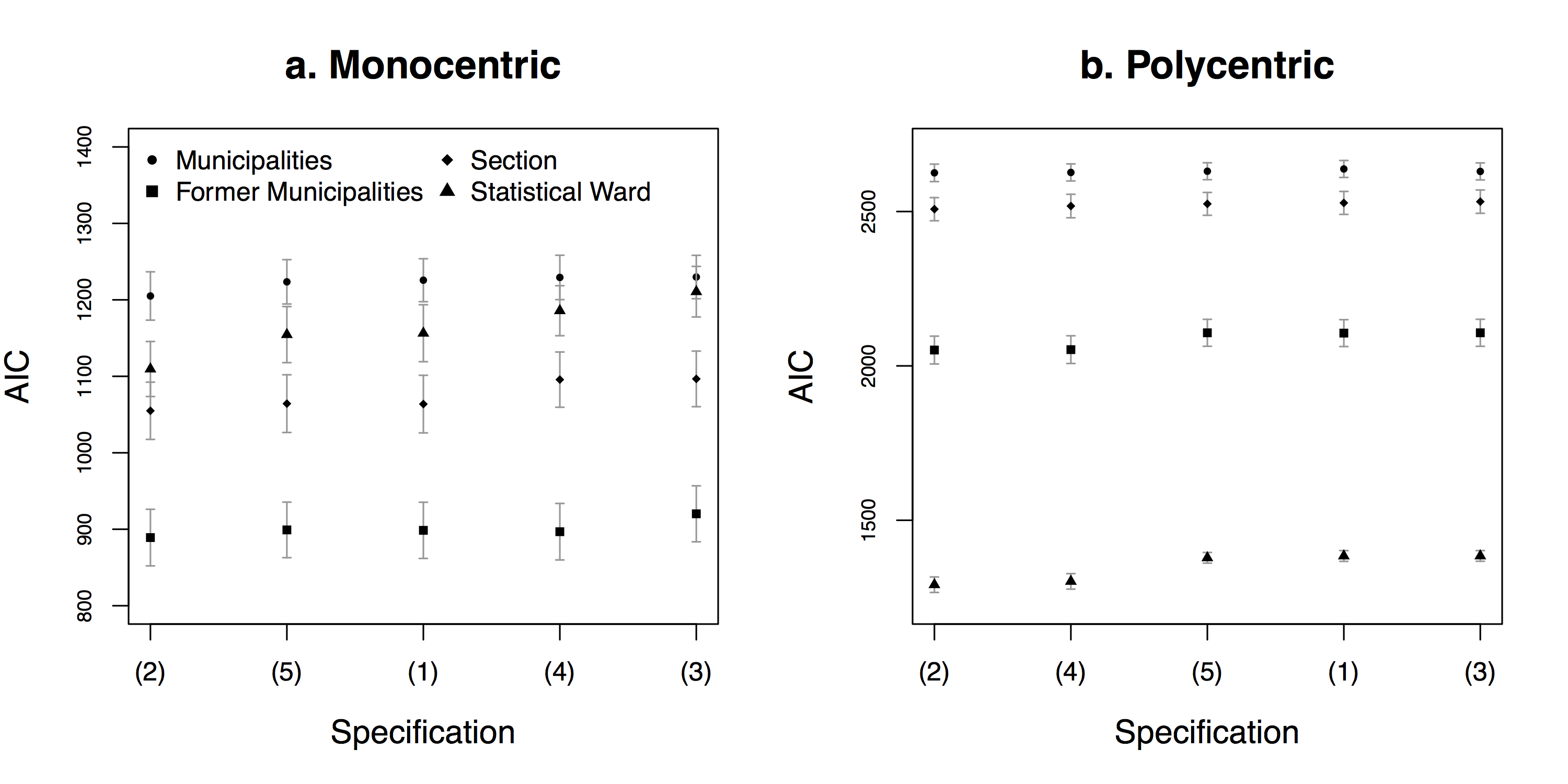
4.1 Selection of the benchmark model
Figure 2 gives AIC values through specifications. For the Monocentric case study, the variations observed across specifications are never significant. Non-significant parameter estimates (see Table 4) are found for specifications (2), (4), and (5). Moreover, specifications (1) and (5) exhibits a multicollinearity problem between the accessibility to jobs and either the distance to highways or the travel time to Brussels, leading to negative parameter estimates for the former variable. Hence, specification (3) will be used as a benchmark for further analysis of the variations through scales, since its goodness-of-fit is similar to those of the other specifications and all the parameter estimates are significant and of the expected sign (i.e. the utility decreases when the distance to Brussels or to the transport infrastructure increases).
For the Polycentric case study, at the statistical ward level, the AIC value is significantly lower for specifications (2) and (4). Non-significant parameter estimates are found for all cases (see Table 5), but less frequently for specifications (2) and (3). The multicollinearity issue remains present, but its magnitude is reduced. Hence, for comparability purpose with the Monocentric case study, it was decided to use specification (3) as a benchmark here as well. Other specifications are used to compare variations linked to the size of the BSUs with the variations between specifications.
Note that the McFadden pseudo R-square (see Tables 4 and 5) of the benchmark model is in most cases slightly lower than the one of specifications (2) and (4). However, the differences remain weak, especially since these specifications include four independent factors instead of three for the benchmark.
4.2 Variations of parameter estimates through BSU level
Across BSU levels, parameter estimates of the benchmark model are significantly different (at the 5% level) for all variables, on all pairs of BSU levels and for both the Monocentric and Polycentric case studies. The only exception is the statistical wards/sections pair for DIST_HGW (results of the pairwise t-test comparisons are given in Table A.1 in Appendix).
Parameter estimates of the benchmark model do not evolve monotonously with the size of the BSUs For the Monocentric case, municipalities appear to behave differently than the three smaller BSU levels, especially for DIST_TRAIN and DIST_HGW (Table 4). For the Polycentric case (Table 5) depending on the variable, statistical wards and municipalities appear different from the other BSU levels. No sign changes are observed among parameter estimates of the benchmark model. It should be noted, however, that TIME_BXL evolves from a non-significant to a positive effect with the size of the BSUs for the Polycentric case study.
4.3 Variations of parameter estimates between specifications
Most parameter estimates are also significantly different between the benchmark model and control specifications for most variables and BSU levels (Table A.2 in Appendix). Non-significant differences appear, however, more frequent, and are mainly observed between the benchmark model and model (4) or (5). The municipalities and sections BSU levels shows more non-significant differences than the two others, without clear explanations. The parameter estimates are also less frequently significantly different for the Polycentric case study than for the Monocentric one, which may be linked to the lower number of jobs.
Sign changes among parameter estimates remain limited, for the Monocentric case study, to the former municipalities level: the parameter estimates of TIME_BXL are positive for model (5), but negative in the benchmark model. The same opposition can be observed for the DIST_TRAIN variable between model (1) and the benchmark. For the Polycentric case, no change of signs can be observed for TIME_BXL and DIST_HGW, only evolutions from significant to non-significant. The DIST_TRAIN variable shows opposite parameter estimates between model (2) and the benchmark at the Former municipalities and Municipalities level. As one could have expected, differences in parameter estimates appear to be linked to the degree of similarity between specifications in terms of variables included (such as the benchmark model and model 4). The inclusion of only one additional variable may, however, have a high influence on parameter estimates, as showed by the pair of specifications (1) and (2), and between the benchmark model and model (5).
| Specifications | |||||||
|
Basic Spatial Units |
Variables |
(1) |
(2) | (3) |
(4) |
(5) | |
| (Benchmark) | |||||||
| Statistical wards | POP_DENS | -0.48*** (0.09) | -0.83*** (0.07) | ||||
| (n BSU = 2074) | ACC_JOBS | -0.39** (0.09) | 3.33*** (0.40) | -0.39** (0.09)
| |||
| (n Jobs = 341 921) | TIME_BXL | -0.26* (0.09) | -0.12*** (0.02) | 3.01*** (0.44)
| |||
| DIST_TRAIN | 2.59*** (0.36) | -0.17*** (0.02) | -0.69*** (0.07) | -0.33** (0.09) | ns
| ||
| DIST_HGW | -0.49*** (0.09) | -0.34* (0.09) | -0.78*** (0.07) | -0.70*** (0.07) | -0.49*** (0.09)
| ||
| Rho2 | 0.48 | 0.5 | 0.46 | 0.47 | 0.48
| ||
| Section | POP_DENS | -0.58*** (0.10) | -0.89*** (0.09) | ||||
| (n BSU = 550) | ACC_JOBS | -0.44** (0.11) | 3.06*** (0.43) | -0.44** (0.11)
| |||
| (n Jobs = 341 921) | TIME_BXL | -0.55*** (0.12) | ns | 2.84*** (0.54)
| |||
| DIST_TRAIN | 2.57*** (0.39) | -0.11* (0.03) | -0.72*** (0.09) | -0.59*** (0.12) | ns
| ||
| DIST_HGW | -0.61*** (0.10) | -0.42** (0.11) | -0.87*** (0.09) | -0.73*** (0.09) | -0.60*** (0.10)
| ||
| Rho2 | 0.52 | 0.53 | 0.51 | 0.51 | 0.52
| ||
| Former municipalities | POP_DENS | -0.64** (0.12) | -0.81*** (0.11) | ||||
| (n BSU = 173) | ACC_JOBS | -0.49* (0.14) | 2.39*** (0.52) | -0.48* (0.14)
| |||
| (n Jobs = 341 921) | TIME_BXL | -1.04*** (0.15) | 0.30*** (0.06) | 2.97** (0.67)
| |||
| DIST_TRAIN | 3.26*** (0.46) | 0.21* (0.06) | -0.76*** (0.12) | -0.74** (0.18) | ns
| ||
| DIST_HGW | -0.65** (0.13) | -0.55** (0.15) | -0.97*** (0.11) | -0.73*** (0.13) | -0.66** (0.13)
| ||
| Rho2 | 0.6 | 0.6 | 0.59 | 0.6 | 0.59
| ||
| Municipalities | POP_DENS | ns | -0.59*** (0.12) | ||||
| (n BSU = 62) | ACC_JOBS | ns | 5.17*** (0.76) | ns
| |||
| (n Jobs = 341 921) | TIME_BXL | -1.09*** (0.20) | ns | 1.86* (0.69)
| |||
| DIST_TRAIN | 2.73*** (0.50) | -0.45*** (0.09) | -0.59** (0.14) | -1.20*** (0.22) | ns
| ||
| DIST_HGW | -0.39* (0.13) | ns | -0.55*** (0.12) | -0.62** (0.14) | -0.41* (0.13)
| ||
| Rho2 | 0.49 | 0.46 | 0.45 | 0.45 | 0.45
| ||
| Specifications | |||||||
|
Basic Spatial Units |
Variables |
(1) |
(2) | (3) |
(4) |
(5) | |
| (Benchmark) | |||||||
| Statistical wards | POP_DENS | -0.59*** (0.08) | -0.64*** (0.08) | ||||
| (n BSU = 4223) | ACC_JOBS | -0.33** (0.07) | 0.87* (0.26) | -0.32** (0.08)
| |||
| (n Jobs = 65 810) | TIME_BXL | ns | -0.22*** (0.02) | 0.96* (0.37)
| |||
| DIST_TRAIN | ns | -0.24*** (0.02) | -0.41*** (0.07) | ns | ns
| ||
| DIST_HGW | -0.46*** (0.07) | -0.32** (0.08) | -0.49*** (0.07) | -0.46*** (0.07) | -0.46*** (0.07)
| ||
| Rho2 | 0.36 | 0.4 | 0.36 | 0.39 | 0.36
| ||
| Section | POP_DENS | -0.86*** (0.06) | -0.87*** (0.06) | ||||
| (n BSU = 1217) | ACC_JOBS | -0.35*** (0.06) | 0.64* (0.19) | -0.34*** (0.06)
| |||
| (n Jobs = 65 810) | TIME_BXL | ns | -0.11** (0.02) | 0.83* (0.29)
| |||
| DIST_TRAIN | ns | -0.12*** (0.02) | -0.42*** (0.06) | ns | ns
| ||
| DIST_HGW | -0.80*** (0.06) | -0.35*** (0.06) | -0.82*** (0.06) | -0.44*** (0.05) | -0.80*** (0.06)
| ||
| Rho2 | 0.41 | 0.42 | 0.41 | 0.41 | 0.41
| ||
| Former municipalities | POP_DENS | -0.77*** (0.07) | -0.78*** (0.07) | ||||
| (n BSU = 473) | ACC_JOBS | -0.86*** (0.08) | ns | -0.86*** (0.08)
| |||
| (n Jobs = 65 810) | TIME_BXL | ns | 0.34*** (0.05) | ns
| |||
| DIST_TRAIN | ns | 0.36*** (0.05) | -0.89*** (0.08) | ns | ns
| ||
| DIST_HGW | -0.95*** (0.07) | -0.94*** (0.09) | -0.95*** (0.07) | -0.90*** (0.08) | -0.95*** (0.07)
| ||
| Rho2 | 0.51 | 0.52 | 0.51 | 0.52 | 0.51
| ||
| Municipalities | POP_DENS | -0.75*** (0.09) | -0.80*** (0.09) | ||||
| (n BSU = 126) | ACC_JOBS | -0.94*** (0.10) | -2.22*** (0.33) | -0.94*** (0.10)
| |||
| (n Jobs = 65 810) | TIME_BXL | 0.75*** (0.11) | ns | ns
| |||
| DIST_TRAIN | -1.36*** (0.23) | 0.27** (0.07) | -0.93*** (0.09) | 0.89*** (0.13) | ns
| ||
| DIST_HGW | -0.83*** (0.08) | -0.99*** (0.10) | -0.85*** (0.08) | -0.91*** (0.09) | -0.85*** (0.08)
| ||
| Rho2 | 0.39 | 0.39 | 0.39 | 0.39 | 0.39
| ||
4.4 Spatial structure of the predicted probability of location
Using the benchmark model, highest probabilities of location are found in the Brussels city centre for both BSUs and case studies, which is consistent with the sign of parameter estimates (Tables 4 and 5). Other clusters of BSUs with high probabilities of location can be observed close to train stations and/or highways (the combination of both factors corresponding usually to a secondary city). Variations in the spatial structure of the probability of location through BSU levels can also be observed on the maps of the predicted probability of location (Figure 3).
If we aggregate the predicted probability of location by statistical ward to municipalities’ level, by summing the probability of all statistical wards belonging to the same municipality, the resulting value is not equal to the probability of location predicted at the level of the municipalities. Relative differences went from -336 to +88% for the Monocentric case study (mean = -21%), and from -324 to +86% for the Polycentric one (mean = -18%). Moreover, the correlation (Pearson) between original and aggregated values is medium: 0,61*** for Monocentric and 0,52*** for Polycentric. And between the relative variations through scales and the predicted probability, non-significant or low correlations are observed (0,19 and 0,24**, respectively).
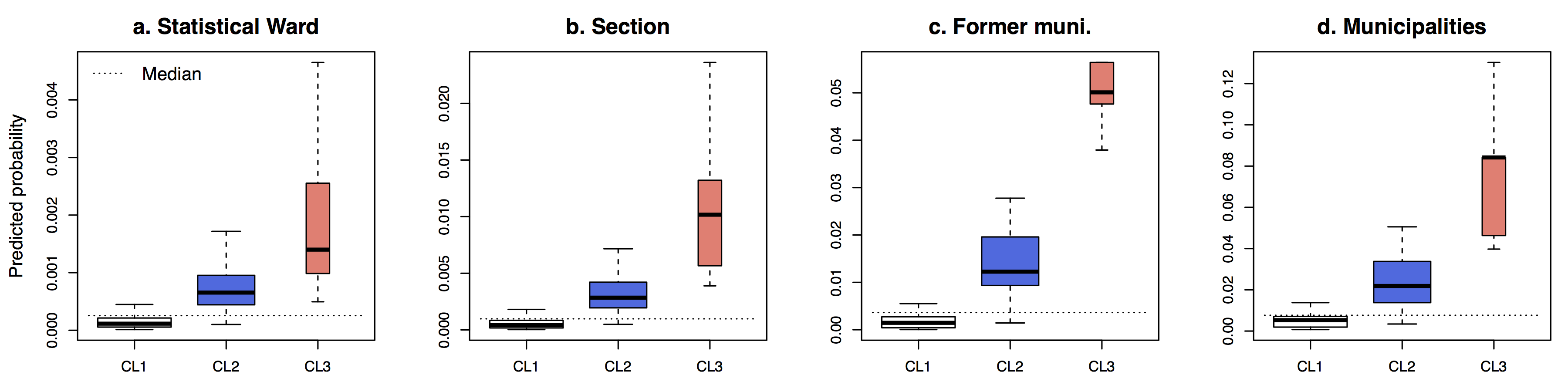
Hence, to explore these variations on a consistent way for the entire study area, a clustering procedure was conducted. For the Monocentric case study, three clusters are obtained. They are organized in concentric rings around the centre of Brussels (Figure 4) and correspond respectively to relatively low (CL1m), medium (CL2m), and high (CL3m) probabilities of location (see Figure A.2 in Appendix). Probabilities are significantly weaker in CL1m than in CL2m, and in CL2m compared to CL3m, for all BSU levels (at α = 0,05).
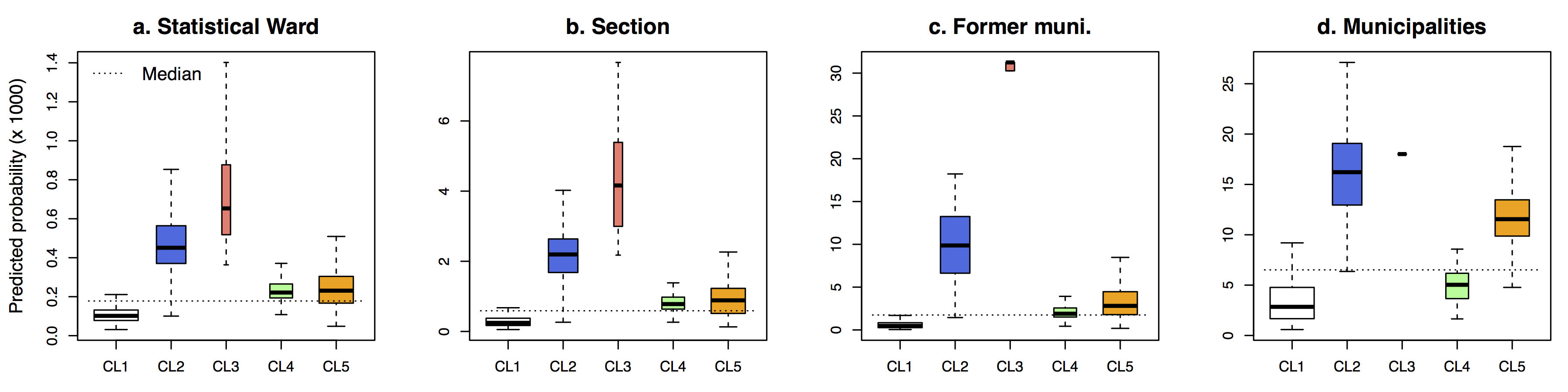
For the Polycentric case study, the clustering produces five clusters. Although the concentric structure from high to low probabilities also appears, with CL3p being the city centre of Brussels, CL1p rural areas, and CL2p suburbs or secondary centers (Figure 4). Two particularities should be noted: CL4p and CL5p have similar values for smaller BSUs, but relatively low values are observed at the municipalities level for CL4p, and the opposite for CL5p (Figure A.3 in Appendix).
Note that for other specifications, the number of clusters (using the exact same procedure) varies from four (model 2 and 5) to ten (model 4) for the Monocentric case study, and from four (model 5) to eleven (model 4) for the Polycentric one. The spatial pattern is also similar, although variations in the number of clusters make a formal comparison difficult.
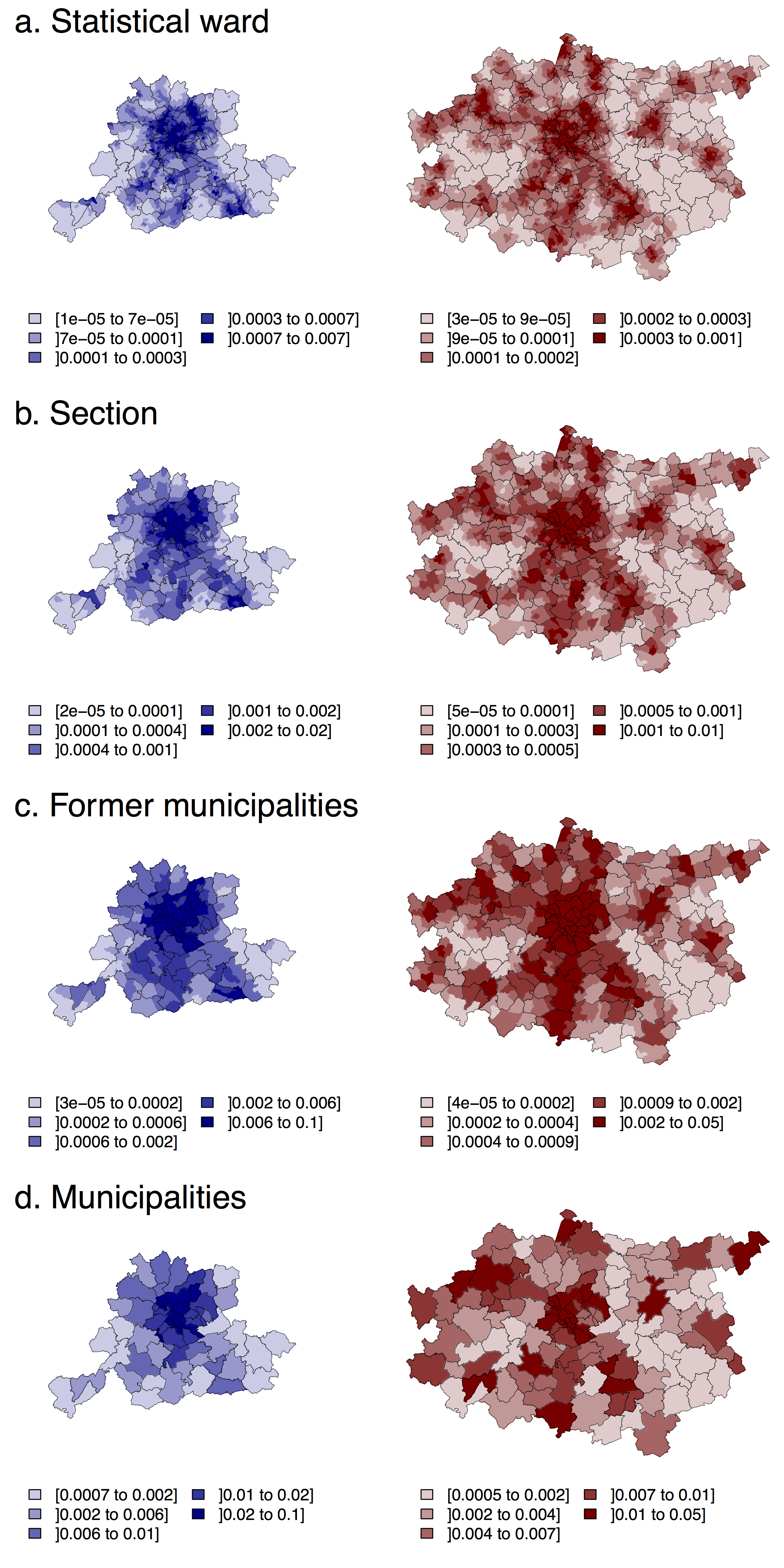
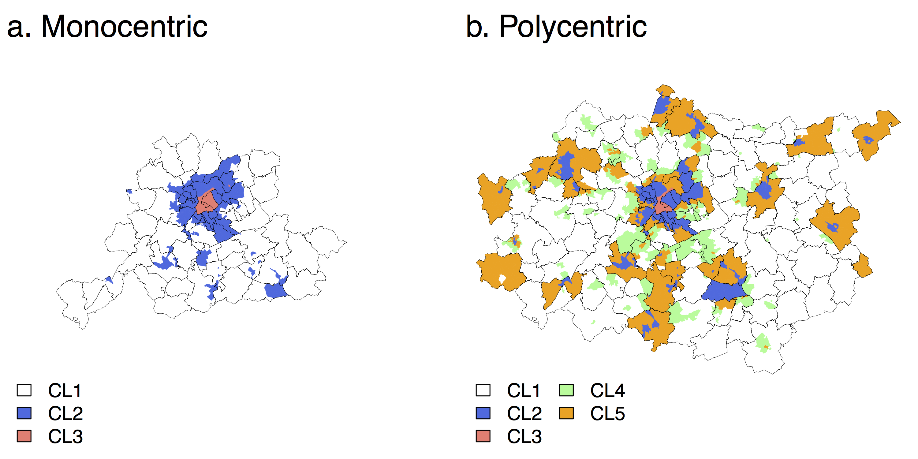
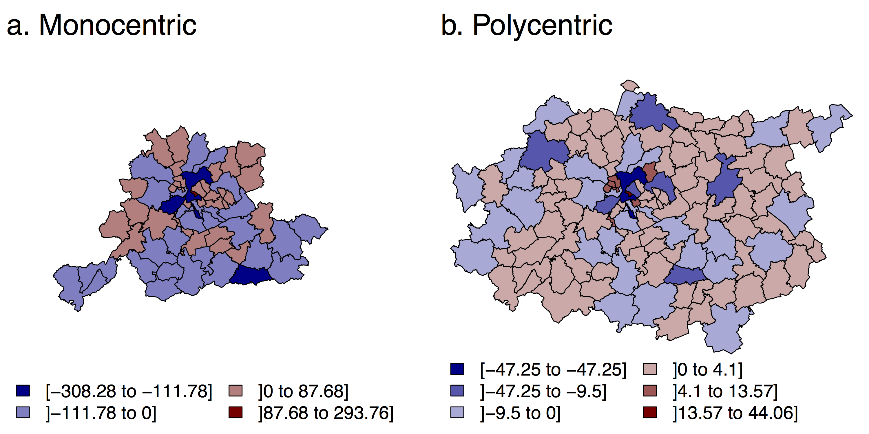
Figure 5 shows the differences in the predicted number of “new” jobs between municipalities and statistical wards. Negative differences mean that more “new” jobs are predicted at the statistical wards level than at the municipalities level, and positive differences the opposite. The spatial structure of the variations is similar for the two activity sectors, which was expected since identical specifications are used, and the parameter estimates are of the same sign. The correlation (Pearson) between the number of new jobs predicted by statistical wards and municipalities is of 0,62*** for the Monocentric case study, and also of 0,62*** for the Polycentric case study. Greater variations are found for the former. They can be explained by the larger number of “new” jobs (3.419 versus 658) and by the lower number of BSU (62 versus 126). The municipality of Brussels and secondary cities receives fewer jobs at the municipality level than at the statistical ward level. On the contrary, more jobs are distributed (at the municipalities level) in different small municipalities within the Brussels-Capital Region. In suburban or rural areas, the differences are limited in magnitude. Negative differences are found for municipalities close to transportation infrastructure, and positive differences for more peripheral municipalities. Hence, for our benchmark model, the concentration of jobs in cities appears to decrease with the size of the BSU.
5 Discussion
5.1 Consistency and limitations
The sensitivity analysis presented in this paper suffers several shortcomings that should be mentioned. The literature shows that the econometric model used (linear-in-parameter MNL model) is subject to many limitations when applied on spatial choice sets (see Section 2). We specifically decided to stick to this model since it is the one used by many LUTI models. Nevertheless, one may wonder if the best option would not be to incorporate LUTI model’s specifications, allowing us to take into account spatial effect (see e.g Guo, Bhat 2004, 2007, Sener et al. 2011, Alamá-Sabater et al. 2011); or use nested logit models. Another drawback is that the specification of the model is limited to simple variables and is identical for all BSU level, although Arauzo-Carod, Manjón-Antolín (2004), de Palma et al. 2007 and our own findings show that location choice factors do not act uniformly through scales. It can thus be argued that specifications tailored for each BSU level could reduce the variations in the spatial structure of the probability of location. Still, the choice of keeping the same specification for all BSU level comes from the fact that the benchmark model performs better at all scales than any other estimated specifications.
Operational implications, for LUTI models, of the sensitivity of DCM to the size of the BSUs can only be partially explored by the stand-alone DCM presented in this paper. The main reason is that the utility of each BSU is assumed here to be constant. There is no feedback effect decreasing the utility of one BSU when its number of jobs increases. In a complete LUTI model, feedbacks can arise from several factors. For instance, if the job density is used as an independent variable with a negative parameter estimate, an increase in the number of jobs in one BSU in t0 will decrease the utility of this BSU in t + 1. Another potential feedback is that the travel time to Brussels may increase when the number of jobs increase due to congestion effect simulated by the transport component of the LUTI model. If such feedbacks are present, the distribution of “new” jobs by a LUTI model would not be identical to the one simulated here.
5.2 Sensitivity of DCMs to the size of the BSUs
The variations observed among parameter estimates between BSU level were expected, given previous works on the MAUP (Amrhein 1995, Arbia 1989, Fotheringham, Wong 1991; for DCM see Arauzo-Carod, Manjón-Antolín 2004, de Palma et al. 2007. This work thus confirms that such variations can be expected in all applications of DCM. Moreover, the size of the BSUs does not influence the sign of parameter estimates, meaning that the influence of a given factor on utility remains positive or negative through scales, but that its intensity varies. This latter result can also be observed in the works of Arauzo-Carod, Manjón-Antolín (2004) and de Palma et al. 2007, which suggest that it may be valid for other applications as well.
On the contrary, the exact direction and magnitude of variations observed in parameter estimates are obviously specific to our case studies: in particular, the absence of regularities in the variations among BSU levels. Depending upon the variable, the highest differences between parameter estimates can be observed between statistical wards and sections (DIST_TRAIN, for the Polycentric case study), between sections and former municipalities (TIME_BXL, for the Monocentric one) or between former and current municipalities (DIST_TRAIN for Monocentric, TIME_BXL for Polycentric). Moreover, these variations are not monotonous: for the Monocentric case study, parameter estimates increase (in absolute terms) between statistical wards and former municipalities, but decrease for municipalities (except for TIME_BXL where a stabilization is observed). For Polycentric, an increase (in absolute terms) is observed between statistical wards and former municipalities, followed by stabilization. Again, there is no indication that this non-monotony can be generalized to other data sets or case studies, since other works assessing the influence of the MAUP on DCM (Arauzo-Carod, Manjón-Antolín 2004, de Palma et al. 2007) rely on only two different levels of analysis.
Hence, predicting or controlling variations of parameter estimates through scale is not straightforward, since these variations do not seem to be directly linked to the size of the BSUs. A potential reason is that administrative units do not correspond to the land-use structure, even if the modellers are often constrained to use such areal units, for data availability reason, and because they remain a relevant unit for policy making. Again, in the absence of comparable analysis in other works, it is difficult to assess the extension of these findings. Since the probability of location in a zone i depends on the utility of i and of all other zones (see Equation 1), we expect that they will remain valid for other case studies.
5.3 Sensitivity of DCMs to misspecification issue
For our case studies, magnitude of the parameter estimates variations are comparable between BSU levels and specifications, since significant differences are observed in most cases (see Tables A.1 and A.2 in Appendix). Contrary to variations across BSU levels, sign change can be observed in parameter estimates and appear to be linked to the correlation structure between explicative factors. Hence, the direction of these variations suggests that differences in parameter estimates between BSU levels and between specifications are not of the same nature.
Previous works (Amrhein 1995, Briant et al. 2010) found larger variations of parameter estimates between specifications than between BSU levels, while here significant differences between pairs of parameter estimates are observed as frequently between BSU levels than between specifications. The use of a different econometric model may constitute an explanation, and scales are not perfectly comparable. Briant et al. (2010), for instance, work on France, and with larger areal units. The high degree of similarity between specifications in terms of independent variables is also likely to reduce the differences between parameter estimates. Hence, in this work, spatial biases are found to be of comparable magnitude with misspecification issues. The location choice models remain here very simple. The comparison of different specification should thus be seen as a methodological precaution (to be sure that spatial biases are worth worrying about), and certainly not as a complete analysis of misspecifications issues in DCM. Hence, this result should be considered as specific to our case studies, rather than as generalizable.
5.4 Influence of scale on the spatial structure of the probability of location
The third research question addressed by this paper focused on if the size of the BSUs influences the spatial structure of the predicted probability of location (let us recall that the case studies correspond to two activity sectors: services and industrial activities). The answer appears to be yes. For instance, the municipality of Ottignies-Louvain-La-Neuve (see Figures 3 and A.1b in Appendix) exhibits, for the Monocentric case study (i.e. for jobs in services), a strong dichotomy between its western part (mostly residential and where low probabilities are observed) and its eastern part (that shows high probabilities), which is close to a highway and currently occupied by an office park. Nevertheless, boundaries of larger BSU level (especially the former municipalities) do not follow this internal structure, which disappears for the larger BSU levels.
More precisely, aggregation into larger BSUs leads either to a “dilution” or, on the contrary, to a “diffusion” of the high probabilities predicted at the statistical wards level. The first process means that statistical wards with a high probability of location are “diluted” when aggregated into larger BSUs, ending up with a municipality having a relatively low probability of location. The second process occurs when the importance of statistical wards with a high probability of location is larger. In this latter case, these high probabilities are “diffused” to the larger BSUs, ending up with a municipality having a relatively high probability of location (as in Ottignies Louvain-La-Neuve).
Results show that these processes have a limited influence for the Monocentric case study, where one cluster corresponds to relatively low probabilities of location at all scales, another to medium probabilities, and the third one to high probabilities. Moreover, the concentric structure of these clusters, centered around the Brussels CBD, is consistent with the urban structure. Statistical wards belonging to the “medium” CL2m cluster that are scattered within the “low” CL1m cluster encompass secondary employment centres (Wavre, Louvain-La-Neuve and Halle). Note that the distribution of the predicted probability of location is highly skewed, which explains why CL2m shows a negative deviation from the global median (Figure A.2 in Appendix).
For the Polycentric case study (i.e. jobs belonging to industrial activities) the situation is more complex. “low”, “medium” and “high” clusters are also found, respectively CL1p, CL2p and CL3p, and their spatial extension are close to the one observed for the Monocentric case. This similarity can be explained by the fact that identical specifications are used for both case studies, and that the parameter estimates are of the same sign. The study area being larger, the “medium” (CL2p) cluster encompasses extra secondary cities: Aalst, Mechelen and Leuven, while the “low” (CL1p) cluster corresponds to most of the rural parts of the study area. Two additional clusters can be observed. CL5p corresponds to statistical wards for which the probability of location is relatively larger for larger BSUs than for the small one, while the opposite situation is observed for CL4p. In terms of spatial structure, CL5p is composed of low-density statistical wards located within the boundaries of the municipalities of the above mentioned secondary employment centres (while the statistical wards where the jobs are actually located in these municipalities belong to CL2p). CL4p is found surrounding isolated CL2p’s statistical wards, or next to CL1p. It is composed of statistical wards that are generally close to spatial units belonging to CL2p, but located on the other side of a municipality boundary. Hence, the relative extension of potential employment centres depends on the scale of the analysis. On the first hand, when the size of the BSU level increases, some statistical wards could become part of an employment centre: this is the “diffusion” process observed for CL5p. On the other hand, some statistical wards are “diluted” into a rural neighbourhood, as for those belonging to CL4p.
5.5 Operational implications and recommendations
The last step in this paper is to assess if the distribution of “new” jobs among BSU levels, proportional to the predicted utility level, varies when observed at different scales. Again, the answer appears to be yes. For our case studies, large differences can be observed in the absolute number of new jobs per municipalities, and a strong spatial structure emerges: the larger BSUs lead to a lower concentration of jobs in urban areas (Figure 5). Hence, even if the experiment performed here shows that the distribution of new jobs is similar through scales (high correlation for the number of new jobs per BSU, see Section 4), it also shows that employment centers can gain more or less importance during the simulation, depending upon the size of the BSUs used.
The nature of the BSUs for which the DCM predicts a high probability of employment location can explain these findings. Such BSUs correspond either to (a) actual employment centers (i.e. a BSU where a large number of jobs are located) or (b) to BSUs having similar intrinsic characteristics as these employment centers, even if the number of jobs located in them is presently small. The latter employment centers are less frequent for larger BSUs than for small one, for two reasons. First, a larger size means that adjacent BSUs are less likely to be exactly similar to each other. Secondly, the lower number of larger BSUs means that the distribution of the probability of location is less continuous. Hence, the spatial heterogeneity increase with the size of the BSUs (although the variation range of independent factors is lower, see Table 2), which may explain the higher heterogeneity in terms of predicted probability of location. However, this spatial heterogeneity does not explain the differences observed when the probability of location at the statistical wards level is aggregated into municipalities (see Section 4.4). Again, these results are specific to our case studies, and we have no indications that they extend to other datasets or case studies.
It is, however, possible to draw from them different recommendations that have a general validity. Stand-alone applications of DCM to study employment location choices will assess the relative importance of each location choice factor (e.g. accessibility, economies of agglomeration, etc.) by comparing parameter estimates. This paper, in line with Arauzo-Carod, Manjón-Antolín (2004) and de Palma et al. (2007), shows that comparing such factors between case studies is extremely risky when areal units of varying size are used.
LUTI models such as UrbanSim or ILUTE rely on the probabilities of location estimated by the DCM to distribute new/relocating agents during iterations of the model. Variations in the spatial structure of the high probability of location thus have important operational implications for land-use planning: they mean that the locations having the best potential for future employment location can change with by the size of the areal units used in the model. These variations in the spatial structure of the probability of location are not straightforward to predict, as showed by the structure of the clusters for the Polycentric case study. The reason is that they depend simultaneously on three elements: (1) the variations of parameter estimates over scales, (2) the variations of the descriptive statistics of the explanative factors, which affect the utility level of each BSU, and (3) the number of these BSUs (the sum of the probability of location is equal to one). Hence, all other things being equal, an increase in the utility of one BSU leads mechanically to a decrease in all others. Given the growing popularity of LUTI models for land-use planning and environmental policy evaluation (see Rodrigue et al. 2009), this potential source of bias in the final situation predicted by a LUTI model should be assessed in further works.
Policy implications are limited, since the lower importance in an employment centre observed for larger BSUs is a result specific to our case studies. However, these case studies correspond to the identification of employment sub centres. Hence, prior to estimating a DCM of employment or firm location choices, a careful exploratory spatial data analysis of the distribution of jobs should be conducted, in order to identify these employment sub centres at different scales and to compare their importance and localization. Even if economic activities still tend to cluster into office parks (Archer, Smith 1993), a multi polarization trend has long been observed in cities (Ladd, Wheaton 1991), and many studies have attempted to identify the sub centres of employment. Nevertheless, no consensus appears on the appropriate methodology (Redfearn 2007): traditional cut-off approach such as in the seminal work of Giuliano, Small (1991) on Los Angeles, locally weighted regressions (McMillen 2001, McMillen, Smith 2003), local measure of spatial autocorrelation (LISA, see Anselin 1995, Riguelle et al. 2007) or DCM used on Dallas-Fort Worth (Shukla, Waddell 1991). Given the sensitivity of econometric method parameter estimates to the size of the areal units demonstrated in the literature, the use of non-parametric methods (such as the LISA) should be preferred.
6 Conclusion
This paper provides an analysis of the sensitivity of Discrete Choice Model to the size of the spatial units used as the choice set. The findings are consistent with the literature on the Modifiable Areal Unit Problem (see Arbia 1989, Fotheringham, Wong 1991) and can be summarized as follows: First, a significant influence to the size of the BSUs is found for parameter estimates of the DCM and, consequently, on the predicted probability of selection of the alternatives in the choice set. It allows for extending previous work (Arauzo-Carod, Manjón-Antolín 2004, de Palma et al. 2007) to a broader range of scales, by showing that similar conclusions can be drawn from an urban case study with a smaller BSUs. Secondly, these variations are of the same order of magnitude than those observed between specifications. If we compare these results to those of Amrhein (1995) or Briant et al. (2010) , it suggests that the relative importance of spatial biases and misspecifications issues depends on the case study and econometric methods considered. Here, a comparable influence on the model is found. Finally, the distribution of new jobs among the study area (using the probability of location predicted by the DCM) is different between scales, meaning that potential employment centers vary with the size of the BSUs.
These results, especially the latter one, have different operational implications. DCM are used to forecast agents’ location choices in many LUTI models (see Wegener 2004). Their outputs (e.g. the final number of jobs and households per BSU) may thus be affected by using one level of BSU instead of another. Since such models are used to assess a wide variety of land-use and/or transportation policies (Rodrigue et al. 2009), these assessments may be affected by the size of the BSUs used in the LUTI model. However, to our knowledge, the sensitivity of LUTI models to the size of the areal units has, until now, not been controlled, and should be assessed for in further works. More direct implication can also be highlighted. For instance, the recommended location of future business parks may be affected by the size of the BSUs used in the model. Hence, ignoring spatial biases may lead to wrong-headedness in policy recommendations. A careful exploratory analysis should be conducted prior to estimating the model to avoid these problems. Overall, this paper shows that an excellent knowledge of the study area is vital for modelling employment location choice, not only of the structure of the economy, but also of the spatial structure of the study area and of the process modelled.
References
Alamá-Sabater L, Artur-Tur A, Navaro-Azorín J (2011) Industrial location, spatial discrete choice models and the need to account for neighbourhood effects. The Annals of Regional Science 47: 393–418
Amrhein CG (1995) The search for the elusive aggegation effect: evidence from statistical simulations. Environment and Planning A 27: 105–119
Anselin L (1995) Local indicators of spatial association – LISA. Geographical Analysis 27: 93–115
Arauzo-Carod JM, Liviano-Solis D, Manjón-Antolín M (2010) Empirical studies in industrial location: an assessment of their methods and results. Journal of Regional Sciences 50: 685–711
Arauzo-Carod JM, Manjón-Antolín M (2004) Firm size and geographical aggregation: an empirical appraisal in industrial location. Small Business Economics 22: 299–312
Arbia G (1989) Statistical effects of spatial data transformations: a proposed general framework. Taylor and Francis, London
Archer W, Smith M (1993) Why do suburban offices cluster? Geographical Analysis 25: 53–64
Baudewyns D (1999) La localisation intra urbaine des firmes: une estimation logit multinomiale. Revue d’économie Régionale et Urbaine 5: 915–930
Baudewyns D, Sekkat K, Ben-Ayad M (2000) Infrastructure publique et localisation des entreprises à Bruxelles et en Wallonie. In: Beine M, Docquier F (eds), Convergence des regions: cas des regions belges. De Boeck, Bruxelles
Ben Akiva ME, Lerman SR (1985) Discrete choice analysis: theory and application to travel demand. MIT Press, Cambridge
Briant A, Combes PP, Lafourcade M (2010) Dots to boxes: do the size and shape of spatial units jeopardize economic geography estimations? Journal of Urban Economics 67: 287–302
Cabrita I, Gayda S, Hurtubia R, Efthymiou D, Thomas I, Peeters D, Jones J, Cotteels C, Nagel K, Nicolai T, Röder D (2015) Integrated land use and transport microsimulation for Brussels. In: Bierlaire M, de Palma A, Hurtubia R, Waddell P (eds), Integrated transport and land use modelling for sustainable cities. EPFL Press, Lausanne
Calinski T, Harabasz J (1974) A dendrite method for cluster analysis. Communications in Statistics - Theory and Methods 3: 1–27
Cavailhès P, Thomas I (2012) Are agricultural and developable land prices governed by the same spatial rules? The case of Belgium. Canadian Journal of Agricultural Economics 61: 439–463
Cheshire P (2010) Why Brussels needs a city-region for the city. Mimeo, Url: http://www.rethinkingbelgium.eu/rebel-initiative-files/ebooks/ebook-7/Cheshire.pdf
Cornelis E, Barthelemy J, Pauly X, Walle F (2012) Modélisation de la mobilité résidentielle en vue d’une micro-simulation des evolutions de population. Les Cahiers Scientifiques du Transport 62: 65–84
Croissant Y (2012) mlogit: multinomial logit model. R package, version 0.2-3, Url: http://CRAN.R-project.org/package=mlogit
de Palma A, Motamedi K, Picard N (2007) Accessibility and environmental quality: inequality in the paris housing market. European Transport / Trasporti Europei 36: 47–74
DGSIE – Direction Générale Statistique et Informations économiques (2013) Nace-bel. Url: http://statbel.fgov.be/fr/statistiques/collecte˙donnees/nomenclatures/nacebel/ accessed June 9, 2015
Duda RO, Hart PE (1973) Pattern classification and scene analysis. John Wiley and Sons, Chichester, UK
Dujardin C, Thomas I, Tulkens H (2007) Quelles frontières pour Bruxelles? Une mise à jour. Reflets et Perspectives de la Vie économique 46: 155–176
Fotheringham AS, Brundson C, Charlton M (2000) Quantitative geography: perpectives on spatial data analysis. Sage Publications Ltd
Fotheringham AS, Wong DW (1991) The modifiable areal unit problem in multivariate statistical analysis. Environment and Planning A 23: 1025–1044
Giuliano G, Small K (1991) Subcenters in the Los Angeles region. Regional Science and Urban Economics 21: 163–182
Goffette-Nagot F, Reginster I, Thomas I (2011) Spatial analysis of residential land prices in Belgium: accessibility, linguistic border, and environmental amenities. Regional Studies 45: 1253–1268
Guimaraes P, Figueiredo O, Woodward D (2004) Industrial location modelling: extending the random utility framework. Journal of Regional Science 44: 1–20
Guo J, Bhat C (2004) Modifiable areal unit: a problem or a matter of perception in the context of residential location choice modelling? Transportation research board conference
Guo J, Bhat C (2007) Operationalizing the concept of neghbourhood: application to residential location choice analysis. Journal of Transport Geography 15: 31–45
Hayter R (1997) The dynamics of industrial location: the factory, the firm and the production system. Technical report, Chichester, UK
Hunt J, Abraham J, De Silva D (2009) Pecas theoretical formulation. Url: http://www.hbaspecto.com/pecas/downloads/
Hunt JD, Miller EJ, Kriger DS (2005) Current operational urban land-use transport modelling frameworks. Transport Reviews 25: 329–376
Jones J, Peeters D, Thomas I (2015) Is cities delineations a prerequisite for urban modelling? The example of land prices determinants in Brussels. Cybergeo: revue européenne de géographie: http://cybergeo.revues.org/26899
Ladd H, Wheaton W (1991) Cause and consequences of the changing urban form. Regional Science and Urban Economics 21: 157–162
Landis J, Zhang M (1998a) The second generation of the California urban futures model. Part 1: model logic and theory. Environment and Planning B: Planning and Design 25: 657–666
Landis J, Zhang M (1998b) The second generation of the California urban futures model. Part 2: specification and calibration results of the land-use change sub model. Environment and Planning B: Planning and design 25: 795–824
Marissal P, Medina-Lockhart P, Vandermotten C, van Hamme G (2006) Les structures socio-économiques de l’espace belge. Monographie de l’Enquête socio-économique générale 2001, Url: http://statbel.fgov.be/fr/modules/publications/statistiques/enquetes_et_methodologie/monographies_de_l_enquete_socio-economique_2001.jsp, Bruxelles
McCann P, Sheppard S (2003) The rise, fall and rise again of industrial location theory. Regional Studies 37: 649–663
McFadden D (1978) Modelling the choice of residential location. In: Karlqvist A, Lundqvist L, Snickars F, Weibull J (eds), Spatial interactions theory and planning models. North Holland, Amsterdam
McMillen DP (2001) Nonparametric employment subcenters identification. Journal of Urban Economics 50: 448–473
McMillen DP, Smith S (2003) The number of subcenters in large urban areas. Journal of Urban Economics 53: 321–338
Meester WJ, Pellenberg PH (2006) The spatial preference map of Dutch entrepreneurs: subjective rating of locations, 1983, 1993 and 2003. Tijdscrijft for Economische en Sociale Geografie 97: 364–376
Moniteur Belge (2004) Ordonnance portant assentiment à la Convention du 4 avril 2003 entre l’état Fédéral, la Région flamande, la Région wallone et la Région de Bruxelles-Capitale visant à mettre en oeuvre le programme du réseau express régional de, vers, dans et autour de Bruxelles. Url: http://www.ejustice.just.fgov.be/cgi/welcome.pl
Nicolas JP, Bouvard A, Million F, Homocianu M, Toillier F, Zucarello P (2008) La localisation des activités économiques au sein de l’Aire Urbaine de Lyon. Laboratoire d’économie des transports, Url: http://simbad.let.fr/localisations/, Lyon
Noth M, Borning A, Waddell P (2003) An extensible modular architecture for simulating urban development, transportation and environmental impact. Computer, Environment and Urban Systems 27: 181–203
ONSS – Office National de la Sécurité Sociale (2015) Statistiques en lignes: Données statistiques concernant l’emploi par lieu de travail compléments. Url: http://www.rsz.fgov.be/fr/statistiques/statistiques-en-ligne/donnees-statistiques-concernant-lemploi-par-lieu-de-travail-compl accessed June 9, 2015
Openshaw S, Taylor PJ (1979) A million or so correlation coefficients: three experiments on the modifiable areal unit problem. In: Wrigley N (ed), Statistical applications in the spatial sciences. Pion, London
Pagliara F, Wilson A (2010) The state-of-the-art in building residential location models. Residential Location Choice 1: 1–20
Redfearn C (2007) The topography of metropolitan employment: Identifying centers of employment in a polycentric urban area. Journal of Urban Economics 61: 519–541
Riguelle F, Thomas I, Verhetsel A (2007) Measuring urban polycentrism: A European case study and its implications. Journal of Economic Geography 7: 193–215
Rodrigue JP, Comtois C, Slack B (2009) The geography of transport systems. Routledge, New York
Salvini PA, Miller EJ (2005) ILUTE: An operational prototype of comprehensive micro simulation model of urban systems. Networks and Spatial Economics 5: 217–234
Sarle WS (1983) Cubic clustering criterion. SAS technical report a-108, SAS Institute Inc. Url: https://support.sas.com/documentation/onlinedoc/v82/techreport˙a108.pdf
Sener I, Pendyala R, Bhat C (2011) Accomodating spatial correlation across choice alternatices in discrete choice models: An application to modelling residential location choice behavior. Journal of Transport Geography 19: 294–303
Shukla V, Waddell P (1991) Firm location and land use in discrete urban space: A study of the spatial structure of Dallas-Fort Worth. Regional Science and Urban Economics 21: 225–253
Thill JC (1992) Choice set formation for destination choice modelling. Progress in Human Geography 16: 361–382
Thisse JF, Thomas I (2007) Bruxelles et Wallonie: une lecture en terme de géo économie urbaine. Reflets et Perspectives de la Vie économique 46: 75–93
Thisse JF, Thomas I (2010) Bruxelles au sein de l’économie belge: un bilan. Reflets et Perspectives de la Vie économique 80: 1–18
Train K (2003) Discrete choice methods with simulation. Cambridge University Press, Cambridge
van Hecke E, Halleux JM, Decroly JM, Merenne-Schoumaker B (2009) Noyaux d’habitats et régions urbaines dans une Belgique urbanisée. Monographie de l’enquête socio-économique générale 2001, Bruxelles, Url: http://statbel.fgov.be/fr/modules/publications/statistiques/enquetes_et_methodologie/monographies_de_l_enquete_socio-economique_2001.jsp
van Malderen L, Jourquin B, Vanoutrive T, Verhetsel A, Witlox F (2012) On the mobility policies of companies: what are the good practices? The Belgian case. Transport Policy 21: 10–19
Vandenbulcke G, Steenberghen T, Thomas I (2007) Accessibility indicators to place and transport. Politique scientifique fédérale (BELSPO), Bruxelles, Url: http://www.belspo.be/belspo/organisation/publ/pub_ostc/AP/rAP02_en.pdf
Waddel P, Ulfarsson G, Franklin J, Lobb J (2007) Incorporating land use in metropolitan transportation planning. Transportation Research Part A 41: 382–410
Waddell P (2000) A behavioural simulation model for metropolitan policy analysis and planning: Residential location and housing market components of UrbanSim. Environment and Planning B: Planning and Design 27: 247–263
Waddell P (2002) UrbanSim: Modelling urban development for land use, transportation and environmental planning. Journal of American Planning Association 68: 297–314
Waddell P, Borning A, Noth M, Freier N, Becke M, Ulfarsson G (2003) Microsimulation of urban development and location choices: Design and implementation of UrbanSim. Networks and Spatial Economics 3: 43–67
Wardman M (1988) A comparison of revealed preference and stated preference model of travel behaviour. Journal of Transport Economics and Policy 22: 71–91
Wegener M (2004) Overview of land-use transport models. In: Hensher A, Button K (eds), Transport geography and spatial systems. Pergamon, Kidlington
Wegener M (2011) The IRPUD model. Spiekermann & Wegener Stadt und Regionalforschung, Dortmund. Url: http://www.spiekermann-wegener.com/mod/pdf/AP_1101_IRPUD_Model.pdf
Witlox F, Jourquin B, Thomas I, Verhetsel A, Vande Vijver E, van Malderen L, Vanoutrive T (2011) Assessing and developing initatives of companies to control and reduce commuter traffic. Politique scientifique fédérale (BELSPO), Bruxelles, Url: http://www.belspo.be/belspo/ssd/science/Reports/ADICCT_FinRep_AD.pdf
A Appendix
| p-value | |||||
| Variable | BSU (1) | BSU (2) | Monocentric | Polycentric
| |
| TIME_BXL | Municipalities | Former muni. | 0.05 | ***
| |
| Sections | *** | ***
| |||
| Stat. ward | *** | ***
| |||
| Former muni. | Sections | *** | ***
| ||
| Stat. ward | *** | ***
| |||
| Sections | Stat. ward | *** | ***
| ||
| DIST_TRAIN | Municipalities | Former muni. | *** | ***
| |
| Sections | *** | 0.01
| |||
| Stat. ward | *** | ***
| |||
| Former muni. | Sections | *** | ***
| ||
| Stat. ward | *** | ***
| |||
| Sections | Stat. ward | *** | ***
| ||
| DIST_HGW | Municipalities | Former muni. | *** | 0.001
| |
| Sections | *** | ***
| |||
| Stat. ward | *** | ***
| |||
| Former muni. | Sections | 0.02 | ***
| ||
| Stat. ward | *** | ***
| |||
| Sections | Stat. ward | 0.2 | 1
| ||
| p-value | |||||
| BSU | Variable | Specification | Monocentric | Polycentric
| |
| Municipalities | TIME_BXL | (4) | 0.002 | ***
| |
| (5) | *** | 0.004
| |||
| DIST_TRAIN | (1) | *** | 1
| ||
| (2) | *** | ***
| |||
| (4) | 0.9 | ***
| |||
| (5) | *** | 1
| |||
| DIST_HGW | (1) | *** | 1
| ||
| (2) | *** | ***
| |||
| (4) | 1 | 1
| |||
| (5) | *** | 1
| |||
| Former muni. | TIME_BXL | (4) | *** | ***
| |
| (5) | *** | ***
| |||
| DIST_TRAIN | (1) | *** | 1
| ||
| (2) | *** | ***
| |||
| (4) | *** | ***
| |||
| (5) | *** | 1
| |||
| DIST_HGW | (1) | *** | 0.01
| ||
| (2) | *** | ***
| |||
| (4) | *** | 1
| |||
| (5) | *** | 0.02
| |||
| Section | TIME_BXL | (4) | 0.1 | ***
| |
| (5) | *** | ***
| |||
| DIST_TRAIN | (1) | *** | 0.4
| ||
| (2) | *** | ***
| |||
| (4) | 1 | ***
| |||
| (5) | *** | 1
| |||
| DIST_HGW | (1) | *** | ***
| ||
| (2) | *** | ***
| |||
| (4) | 1 | 0.08
| |||
| (5) | *** | ***
| |||
| Statistical wards | TIME_BXL | (4) | *** | ***
| |
| (5) | *** | ***
| |||
| DIST_TRAIN | (1) | *** | 0.02
| ||
| (2) | *** | ***
| |||
| (4) | *** | ***
| |||
| (5) | *** | ***
| |||
| DIST_HGW | (1) | *** | ***
| ||
| (2) | *** | ***
| |||
| (4) | 1 | ***
| |||
| (5) | *** | ***
| |||