 Volume
4, Number 3, 2017, 1–17 journal homepage:
region.ersa.org
Volume
4, Number 3, 2017, 1–17 journal homepage:
region.ersa.orgDOI: 10.18335/region.v4i3.142
Territory and Sustainable Tourism Development:
A Space-Time Analysis on European Regions
1 University of Algarve, Faro, Portugal (email: jfromao@ualg.pt)2 University of Algarve, Faro, Portugal (email: jguerreiro@ualg.pt)
3 Bank of Portugal and Universidade Nova de Lisboa, Lisbon, Portugal (email: pmrodrigues@bportugal.pt) Received: 8 July 2016/Accepted: 26 April 2017
Abstract. In the long run, tourism competitiveness depends on the sustainable use of territorial assets: the differentiation of destinations depends on the integration of cultural and natural resources into the tourism supply, but also on their preservation over time. Using advanced spatial econometric techniques this work analyses the relationships between regional tourism competitiveness, the dynamics of tourism demand and investment, as well as the existence of natural resources and cultural assets in the European context. Despite the close relationship between tourism activities and the characteristics of the territories, the application of methods of spatial analysis in tourism studies is still scarce and the results of this work clearly show their potential for this field of research. Among the main findings of this paper, it was observed that natural resources do not have the expected positive impacts on regional tourism competitiveness and that European regions with more abundant natural resources are often developing unsustainable forms of mass tourism with low value added and little benefits for the host communities. The existence of spatial correlation effects suggests that positive spillovers arising from tourism dynamics in neighbourhood regions prevail over potential negative effects related to the competition between destinations. Policy and managerial implications of these results are discussed and further research questions are proposed.
Key words: Cultural heritage; Natural resources; Endogenous resources; Spatial autocorrelation; Spatial econometrics; Competitiveness; Sustainability
1 Introduction
As one of the fastest growing sectors in the contemporary global economy, tourism activities face unprecedented levels of competition. However, it is not only a competition between product and service providers, but also between destinations and, consequently, between territories. On the other hand, as tourism attractiveness often relies on territorial natural and cultural endowments, questions related to the sustainable use of these resources assume greater importance as tourism is achieving higher relevance at the international level. This is expressed by the number of tourists worldwide and also by their socio-economic and environmental impacts.
The purpose of this work is to provide a comprehensive analysis of the importance of local resources – both cultural and natural – for regional tourism competitiveness, measured in terms of the gross value added by the tourism sector, at the European level. Our analysis is framed by the concepts of competitiveness and sustainability in tourism. We assume the definition of competitiveness proposed by Ritchie, Crouch (2003), which establishes a clear link to the socio-economic benefits for the local communities and the sustainable use of sensitive territorial resources. Section 2.1 offers a brief literature review for this conceptual framework focusing on the relations between competitiveness and sustainability in tourism.
As our study aims to identify the impacts of tourism on regional socio-economic dynamics, the territorial level of analysis is not exactly the destination, but rather the regional level (NUTS 2, according to the definitions of Eurostat, which is the territorial level typically used for the application of regional policies, while the NUTS 1 level corresponds to the major socio-economic regions and NUTS 3 to small regions). Although these regions normally include more than one tourism destination, they are institutionally relevant in order to address policy questions related to the integration of tourism dynamics into broader resource management or economic development policies. A synthesis of tourism competitiveness studies focused on this territorial level is presented in Section 2.1. In particular, Cucculelli, Goffi (2016) and Cuccia et al. (2016) have analysed similar problems related to natural and cultural resources.
Assuming tourism as a place oriented activity, where territories interact with each other, the possible existence of spatial effects among the regions under analysis is also of interest for the purposes of our study. Despite the close connection between tourism and the territorial characteristics, very few studies have applied spatial econometric methods to the field of tourism as described in Section 2.3. For the purpose of our study, the analysis of the relations between tourism dynamics and cultural assets in Italian regions proposed by Patuelli et al. (2013) or the study of the impacts of natural and cultural endowment on regional tourism demand at the European level developed by Romão (2015) are relevant examples.
Considering that competitiveness implies the creation of high value added and the sustainable use of natural and cultural resources, our paper applies spatial analysis techniques in order to identify different spatial patters in tourism dynamics (Section 3). This analysis is combined with an econometric overall explanation, with the estimation of a general trend within European regions (Section 4). As the work focuses on a large group of regions and considers a period of eight years, a spatial panel data model has been chosen in order to deal with cross-sectional and time series characteristics of the data, while allowing for the identification and quantification of potential spatial effects.
Although limited data availability constrains a comprehensive analysis of all questions related to regional tourism competitiveness, the available information and the methodologies applied in this study contribute to the understanding of the relations over time between attractive and sensitive territorial resources, tourism dynamics and tourism competitiveness at the European regional level. This work provides an innovative analysis of the spatial effects between tourism demand, tourism infrastructures, regional tourism competitiveness and the sustainable use of natural and cultural resources in European regions with relevant results arising from the exploratory spatial analysis and the regression model. A discussion of their policy implications will be presented in the concluding section and issues for further research will be highlighted.
2 Competitiveness, Sustainability and Spatial Econometrics in Tourism
2.1 Tourism competitiveness and sustainable use of resources
The concepts of competitiveness and sustainability emerged in the literature during the 1980s. Michael Porter’s analysis (Porter 1985, 2003) regarding the achievement of a competitive advantage at the firm level had clear implications on economic policy formulations at the regional and national levels. On the other hand, the concept of sustainability was introduced after the publication of the document “Our Common Future” (World Commission on Environment and Development 1987), establishing the principles of sustainable development and taking into consideration its multiple dimensions (economic, social or environmental).
These concepts have been applied to tourism studies during the subsequent years and a good synthesis has been provided in a short note by Poon (1994), by applying some of the generic strategic formulations proposed by Porter and defining a strategy of cost leadership (related to mass tourism, with low value added and high negative externalities) or differentiation (related to the creation of unique experiences, with high value added and low negative externalities, which are understood as corresponding to the concept of sustainability).
This idea would be questioned by Butler (1999) who claims that sustainability and the principles of sustainable development should also be applied to mass tourism development processes, while concerns related to the excessive use of resources are also relevant for small scale forms of tourism in sensitive natural areas. Of particular importance for our work was the distinction proposed by this author between the impacts of tourism on sustainable development and the sustainable use of territorial resources for tourism activities (which is the perspective adopted in our analysis). This conceptualization was supported by Jafari (2001) when defining the “Knowledge Based Platform” for tourism studies who pointed out that principles of sustainability should be addressed at policy and managerial levels in all types of tourism destinations. Both authors emphasised the human dimension of sustainability and the importance of the socio-economic benefits of tourism for the host communities.
During that period, other authors stressed the importance of the uniqueness of local resources for destination differentiation along with the perception and satisfaction achieved by tourists (e.g. Kozak 1999, Buhalis 2000) while bringing attention to the sensitiveness of natural resources and the necessary limits to be imposed to their usage (Buhalis 1999, Hassan 2000). This “environmental paradox”, as later defined by Williams, Ponsford (2009), implies that the production of tourism experiences depends on the exploitation of local resources, which – at the same time – must be preserved.
Synthetizing these contributions, a definition of tourism competitiveness commonly accepted in the literature was provided by Ritchie, Crouch (2003) stating that “what makes a tourism destination truly competitive is its ability to increase tourism expenditure, to increasingly attract visitors, while providing them with satisfying, memorable experiences, and to do so in a profitable way, while enhancing the well-being of destination residents and preserving the natural capital of the destination for future generations”. This definition stresses the importance of growth, economic impacts, consumer satisfaction, benefits for the host community and the preservation of resources over time. Our analysis is particularly focused on the regional economic impacts and the sustainable use of resources.
Following this definition, the authors developed a comprehensive model of destination competiveness while other systematic approaches were proposed in subsequent years (e.g. Vanhove 2005, Mazanek et al. 2007). In particular, Celant (2007) focused his analysis at the regional level, while Weaver (2006), Wall, Mathieson (2006) or Sharpley (2009) offered a more clear focus on the problems of sustainability. Tsai et al. (2009) as well as Park, Jang (2014) offer detailed overviews of these formulations. Systematic approaches combining tourism competitiveness with the principles of sustainable development were proposed as policy guidelines by international institutions like UNESCO (2000, 2005), the European Commission (2007), UNWTO (2007) or the World Economic Forum (2008).
2.2 The region as the territorial level of analysis
Although some of the studies on competitiveness previously mentioned are related to empirical applications focused on particular destinations, most of them aim at international comparisons, which has lead to the creation of country rankings based on composite indicators. One example with large international recognition is the Travel and Tourism Competitiveness Index developed by the World Economic Forum (2008), which uses a very large set of quantitative indicators. Based on this index, several authors applied different methodologies in order to refine the analysis of particular aspects of tourism competiveness: Mazanek et al. (2007) selected a particular group of indicators in order to provide an explanatory model for tourism competitiveness; Navickas, Malakauskaite (2009) oriented the use of these indicators to questions related with innovation; Webster, Ivanov (2014) analysed the relation between this index and the contribution of tourism for economic growth; Martín et al. (2017) proposed a definition of a benchmark position and country profiles regarding tourism competitiveness.
Despite the abundant number of studies on tourism competiveness at the country level, comparative analyses between regions of different countries are relatively scarce, probably due to the difficulties in obtaining relevant and comparable data. Camisón, Forés (2015) focused on the firm level and analysed how regional competitiveness influences the performance of tourism companies. Cracolici, Nijkamp (2008) related the attractiveness of Southern Italian (NUTS 2) regions with tourist satisfaction as a proxy for regional competitiveness. Closer to the purposes of our study, and focusing on a larger number of Italian NUTS 2 regions, Cuccia et al. (2016) observed that cultural and environmental regional endowment positively affect the performance of destinations, but the existence of UNESCO sites does not imply similar benefits. With a different territorial focus (centred on the destination) Cucculelli, Goffi (2016) observed that factors related to the sustainable use of resources exert positive impacts on the performance of Italian certified destinations.
Considering NUTS 2 regions as the territorial level of analysis, our study aims at offering a comprehensive overview of the relations between tourism performance and natural and cultural endowment in order to achieve policy implications both in terms of tourism development and resource management, which are addressed at a relevant institutional level for strategic orientations.
2.3 Spatial econometrics in tourism
Due to the large increment of geo-referenced statistical information recently available and the development of easy-to-use software tools, spatial econometric methodologies are only currently becoming of widespread use even though they started to be developed in the mid 20th century (Florax, Vlist 2003, Anselin 2010). In particular, our work is based on a panel data approach. This allows for the development of complex analyses of economic processes and their spatial effects while taking into consideration more information, increasing the variation and reducing the collinearity between variables resulting in more efficient estimations (Elhorst 2003, 2014).
A limited number of panel data models have been used in tourism studies, mostly over the last 10 years, as summarized by Song et al. (2012). Moreover, despite the close relationship between tourism and territory, only a few works applied spatial panel data models in tourism: Marrocu, Paci (2013) analysed the determinants of tourism flows between 107 Italian locations; Yang, Fik (2014) examined spatial spillovers and spatial heterogeneity in order to explain the variability in tourism growth across 342 cities in China; Kang et al. (2014) analysed the territorial impacts of national tourism policies in South Korea; Ma et al. (2015) focused on the spatial correlation between tourism and urban economic growth in 272 Chinese regions; Majewska (2015) applied techniques of exploratory spatial data analysis to study the inter-regional agglomeration effects in tourism activities in Poland.
Closer to the purpose of our work, Patuelli et al. (2013) examined the importance of world heritage sites on internal tourism flows in Italy, finding positive impacts on the regions where the sites are located followed by negative impacts on tourism flows in the surrounding regions, suggesting the existence of a strong competitive effect. In particular, the results obtained by Romão (2015) in a spatial analysis of the impact of natural and cultural assets on tourism demand in European regions (identifying a positive correlation between the regional endowment on natural and cultural resources and the volume of tourism demand) can be compared with those presented in this paper.
3 Data, methodologies and results
This section includes a presentation of the data and variables under analysis, a preliminary panel regression estimating the impacts of the factors considered on regional tourism competitiveness, an exploratory spatial analysis aiming at the identification of possible spatial effects and, finally, an econometric regression including spatial effects and offering an overall explanatory framework.
3.1 Data and Variables: Tourism Dynamics, Culture and Nature
The territorial level considered in the present study is the NUTS 2 level according to the definitions of the Eurostat for the European regions. This regional scale is appropriate for the purposes of this study as it allows us to obtain relevant and comparable data and to discuss and address policy recommendations at an adequate institutional level. 237 regions (excluding islands) from Austria, Belgium, Bulgaria, the Czech Republic, Denmark, Estonia, Finland, France, Germany, Greece, Hungary, Italy, Latvia, Lithuania, Luxemburg, the Netherlands, Poland, Portugal, Romania, Slovakia, Slovenia, Spain and the United Kingdom have been considered. Other European regions have not been included due to the lack of statistical information. The source for the geographical representation of the data in the following Figures is GISCO – Eurostat (European Commission) for the administrative boundaries of European regions, while the information related to tourism dynamics, cultural assets and natural resources has been added to that source. The maps used in this section (Figures 1 and 2) were produced with QGIS 2.4, while those used in the following section (Figure 3) were produced with GeoDa 1.6.7.
Tourism competitiveness (the dependent variable considered in the spatial panel data model to be developed below) is measured based on available Eurostat data and taking into consideration the gross value added (at current prices) by tourism activities (including wholesale and retail trade; transport; accommodation and food service activities; information and communication services) in each region. This corresponds to a broad definition of tourism services and assumes the increasing importance of information and communication technologies (ICT) for tourism. Some missing data detected for a small number of regions were computed according to the existing information, considering the registered trends immediately before and/or after the missing information.
The explanatory variables considered in the model to be presented include tourism demand (measured by the nights spent at tourism accommodation establishments, according to Eurostat, as a proxy for regional tourism attractiveness) and investment in tourism (gross fixed capital formation in the sector, also based on Eurostat data, as a proxy for the tourism related infrastructures). Natural resources are measured taking into consideration the territory of each region classified by the European Union within the Natura 2000 network (according to a harmonized set of rules and criteria, with the information available at the European Commission – DG Environment), while cultural assets are measured considering the number of World Heritage sites classified by UNESCO at the regional level (also following an international classification based on universal criteria). The evolution between 2004 and 2011 is considered for all these variables.
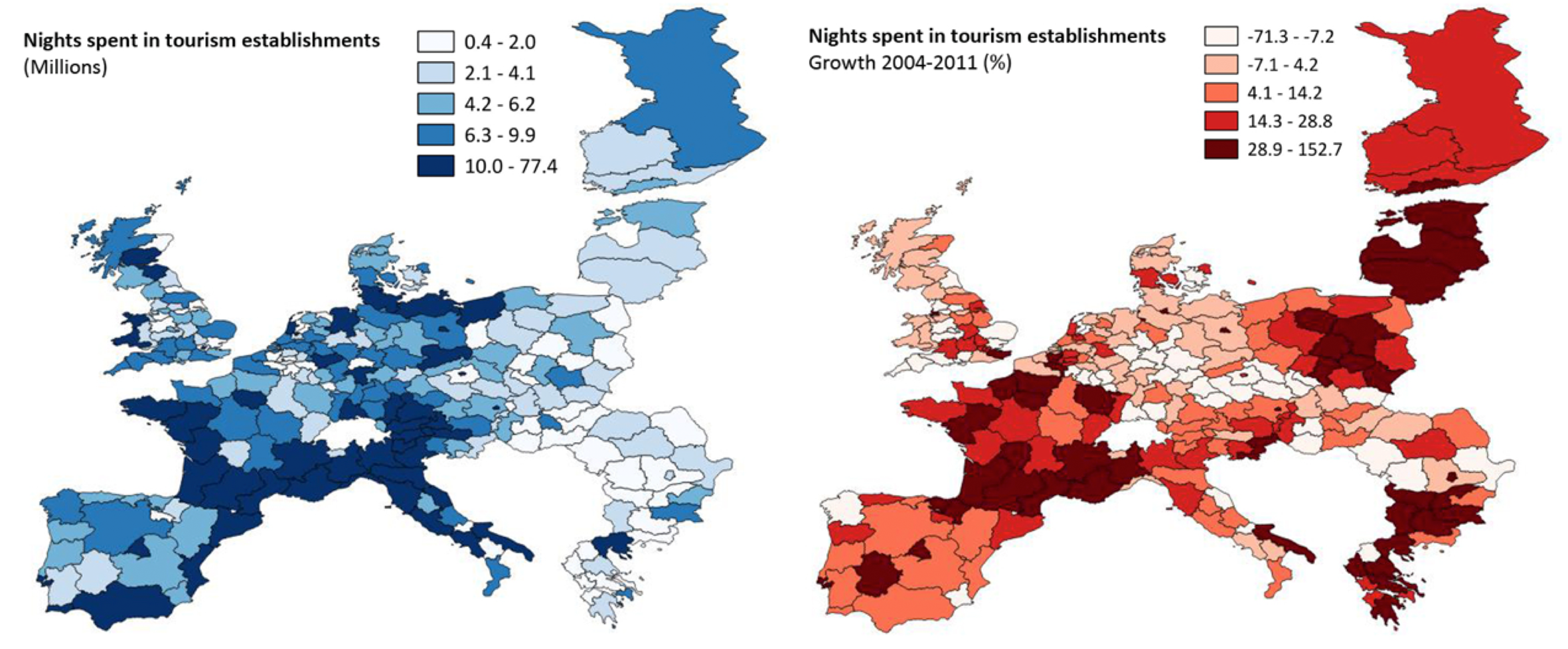
The information for the most recent year (2011) regarding the geographical distribution of tourism demand in European regions measured by the nights spent in accommodation establishments (hotels, holiday and other short-stay accommodation, camping grounds, recreational vehicle parks and trailer parks) is represented in the map on the left hand side of Figure 1, while the growth rates for this indicator between 2004 and 2011 are shown in the right hand side (the classes were created based on quintiles). The spatial pattern identified in Figure 1 reveals the importance of the Southern European regions, but the map on the right hand side of the same Figure reveals a clear shift in tourism demand with a large amount of regions located in the Eastern side of Europe (mostly Baltic, Bulgarian and Greek regions) among those with the highest growth rates registered between 2004 and 2011. However, it should be noticed that these high growth rates are also related to the low scores observed for these regions in the initial period.
The natural resources of each region have been measured taking into consideration the percentage of its territory included in Natura 2000, as a proxy for regional biodiversity. Although these protected areas are not necessarily tourism attractions, they reveal the potential attractiveness of natural resources for tourism demand in each region. In this analysis natural resources are not seen as tourism products, neither is it required that they are perceived as such (or even as protected areas) by tourists: they allow us to assess the sensitiveness and importance of regional ecosystems. The map presented on the left hand side of Figure 2 represents this information for 2011, showing the importance of Southern European regions for the biodiversity in Europe.
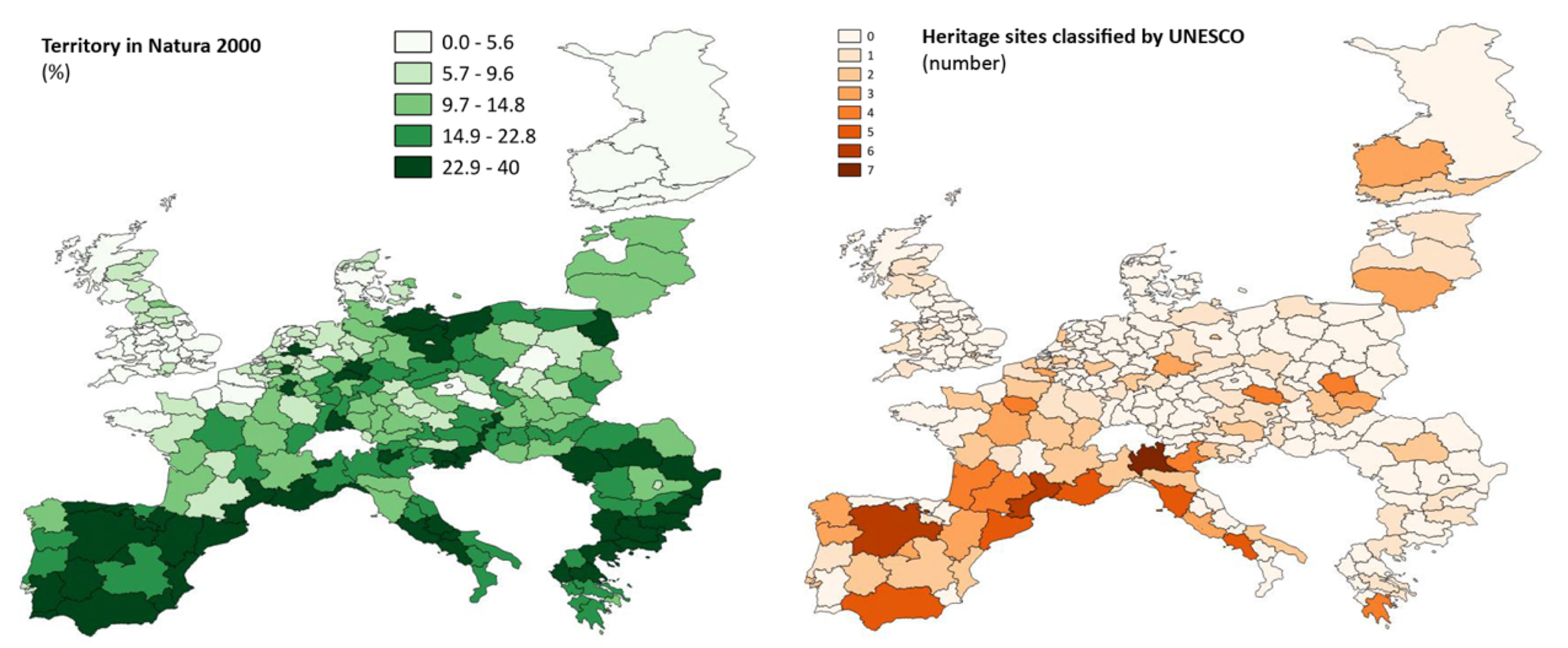
Finally, the number of sites classified as World Heritage by UNESCO in each region was assumed as a proxy for its cultural heritage (in a few cases, the same site is distributed along different regions and one site per region has been considered). Despite the existence of other important cultural elements (from tangible, like non-classified monuments or museums, to intangible, like local lifestyles, and including cultural events and festivals) extremely relevant for tourism attractiveness, it is not possible to have comparable quantitative information at the regional level for an international analysis. The map on the right hand side of Figure 2 represents cultural heritage as measured by the number by UNESCO sites again revealing the importance of the Southern European regions. In the same sense as it was seen for the natural resources, our analysis does not imply the utilization of these assets as tourism products or the perception of their historical importance by tourists: they represent a proxy for the richness of cultural heritage in each region.
3.2 Panel data model without spatial effects
As the purpose of this work is to analyse the effects of tourism demand, investment, natural resources and cultural assets on the regional tourism competitiveness in a large number of European regions over 8 years, a panel data model is an adequate tool. For the purposes of estimation of the models, logarithms are applied to the dependent variable (GVA in the tourism sector – “logGVA”) and to some of the independent variables (such as the number of nights spent in tourism accommodation establishments – “logNIT” – and gross fixed capital formation in the tourism sector – “logINV”), in order to reduce the dispersion of the data. Absolute values are considered for the number of heritage sites (“HERIT”) and percentages for the portion of the territory included in Natura 2000 (“NAT”). No spatial effects are considered in a first stage and the model is specified as:
 | (1) |
where the index i refers to the ith region, t is an index for the time period and u is an independent and identically distributed error term.
Although the number of periods under analysis is relatively small (8 years), the coss-sectionally augmented Im, Pesaran and Shin (IPS) test for panel unit roots (Pesaran 2007) has been applied (using the plm package in R; see Croissant et al. 2016) confirming the stationarity of the data under different test specifications allowing for individual intercepts or trends among the data, defining the number of lags of the test regression according to the Akaike Information Criteria and specifying the maximum number of lags as 2 or 4. The test statistics obtained were, respectively, -51.632 and -61.873, corresponding both to a p-value below 2.2e-16), confirming the stationarity of the data. A variance inflation test (VIF) was also computed (using the package car in R) and all the scores obtained (logNIT = 1.715; logINV = 1.807, NAT = 1.060; HERIT = 1,333) were clearly below the threshold of 5 suggested by O’Brien (2007), revealing the absence of problems of multicollinearity.
In order to choose between a fixed or a random effects model, a Hausman test has been computed with the plm package in R and its result (p-value < 2.2e-16) suggested that a fixed effects model should be preferred (methodologies and techniques are described in Croissant, Millo 2008). Nevertheless, as discussed by Clark, Liner (2015), the Hausman test has important limitations for a final decision regarding the choice of a specific model, which should be grounded on theoretical assumptions about the observations. In our case – and considering the close link between the specific characteristics of the territories and tourism dynamics, it seems plausible to assume that individual regional features have specific impacts on tourism activities, also justifying the option for a fixed effects model. Thus, a panel data model with fixed effects has been estimated.
The estimation results are presented in Table 1, revealing a positive (and statistically relevant) relation between tourism GVA and all the independent variables, except for natural resources. It is possible to confirm the expected positive correlation between the existence of classified heritage sites and tourism competitiveness. It is noticeable that the variables related to tourism dynamics (demand and investment) exert a higher impact on tourism competitiveness than the impact generated by the existence of cultural assets.
| Parameters | Estimate | Std. Error | t-value |
| logNIT | 0.146*** | 0.019 | 6.761 |
| logINV | 0.049*** | 0.010 | 4.823 |
| NAT | -0.003*** | 0.001 | -2.343 |
| HERIT | 0.031*** | 0.013 | 2.396 |
The result related to the negative impact of natural resources on tourism competitiveness requires a more careful interpretation: it could be argued that this negative correlation is the expectable consequence of the fact that natural resources are measured taking into consideration the proportion of protected areas in each region (since the related conservation measures that are implied generally impose restrictions on tourism activities). Nevertheless, as observed in the previous section, these regions are mostly located in Southern Europe, which are generally places with high levels of tourism demand. In fact, a positive relation between tourism demand and the portion of the territory included in Natura 2000 had been found in a previous study on the same regions and for a similar period (Romão 2015).
Thus richer natural resources are correlated to higher levels of demand but to relatively low value added. In other words, despite the apparent potential of these regions to create a differentiated tourism supply, based on their rich biodiversity within the European context, they seem to develop tourism products and services oriented to mass consumption normally with relevant negative consequences in terms of the protection of sensitive environmental resources. Therefore, a strategy of cost leadership (implying a massive use of resources with low economic impact) seems to prevail over a differentiation strategy based on the uniqueness of the places (oriented to the provision of unique experiences with protection of sensitive resources and oriented to high value added products and services).
Despite the high statistical relevance of all parameter estimates of this model, the R-squared (0,048) and the Adjusted R-squared (0,042) obtained from this regression are relatively low. Although the R-squared statistic may have important limitations when applied to time series, the results suggest that the estimation can be significantly improved. Also, the computation (with the plm package for R) of a test (Pesaran CD) for cross-sectional dependence (Pesaran et al. 2008) has lead to results (test statistic of 54.592) suggesting evidence in favour of the existence of such characteristics in the panel under analysis, opening the possibility for the existence of spatial effects.
Finally, as suggested by Clark, Liner (2015), different specifications of the model have been computed in order to confirm the stability of the results. As can be seen from Table A.1 (Appendix) the signs of the estimates for all parameters are the same independently of the type of model (fixed effects, random effects or pooling), although some differences can be observed regarding the statistical relevance of the estimates. On the other hand, a second set of models has been computed (Table A.2 in Appendix) replacing the variables that had been logarithmized (GVA, gross fixed capital formation in the tourism sector, and nights spent in accommodation establishments), which were, instead, divided by the number of residents in each region (values per habitant were obtained) in order to consider the possible effects of the dimension of the region. As can be observed the results show exactly the same signs for all estimates, but with a much lower statistical significance.
3.3 Exploratory Spatial Data Analysis: Territorial Resources and Tourism Competitiveness
In order to identify the possible existence of spatial effects, several preliminary tests were computed by using indicators of spatial autocorrelation (Anselin 2005). This methodology requires the creation of a spatial weights matrix, defining the spatial impacts of each region on its neighbours (Anselin 2005). In this case, a neighbour is defined according to the rook contiguity criteria (two regions are considered neighbours if they share a common border) and it is also assumed that spatial impacts occur, not only for immediate neighbours, but also for the “neighbours of neighbours” (second level contiguity). Additionally, it is also assumed that the impact on immediate neighbours is double than the impact on second order neighbours and that all regions have the same potential to generate spillover effects (implying that the spatial weights matrix is row normalized). The results obtained suggest that this impact matrix offers useful insights for the estimation of spatial effects.
Moran I tests for spatial autocorrelation (Anselin 2005) provide a measure for global spatial correlation between neighbours. Table 2 shows the test results obtained (using Geoda 1.6.0) for all variables included in the model and considers the first and last year of the observations. The existence of spatial correlation is suggested by the test results obtained (a pseudo significance level is computed through a random permutation procedure, recalculated 99 times in order to generate a reference distribution).
| logGVA | logNIG | logINV | HERIT | NAT
| ||||||
| 2004 | 2011 | 2004 | 2011 | 2004 | 2011 | 2004 | 2011 | 2004 | 2011 | |
| Test Results | 8.869 | 9.105 | 10.34 | 11.74 | 6.586 | 9.498 | 6.728 | 8.695 | 16.76 | 18.69 |
Local indicators of spatial autocorrelation have also been computed (with Geoda 1.6.0 and following the methodologies proposed by Anselin 2005) in order to generate a bivariate analysis based on the local Moran I indicators, relating a non-lagged variable (the dependent variable – GVA in tourism) with spatially lagged variables (each of the four independent variables – tourism demand, investment in tourism, natural resources and cultural resources). The maps in Figure 3 represent these spatial relations, considering a 95% significance level. Dark colours represent clusters of positively correlated regions (dark red for high values in both variables and dark blue for low values in both variables) and light colours represent negative correlation (light red for high values of the non-lagged variable and low values for the lagged variable, and light blue for the inverse situation).
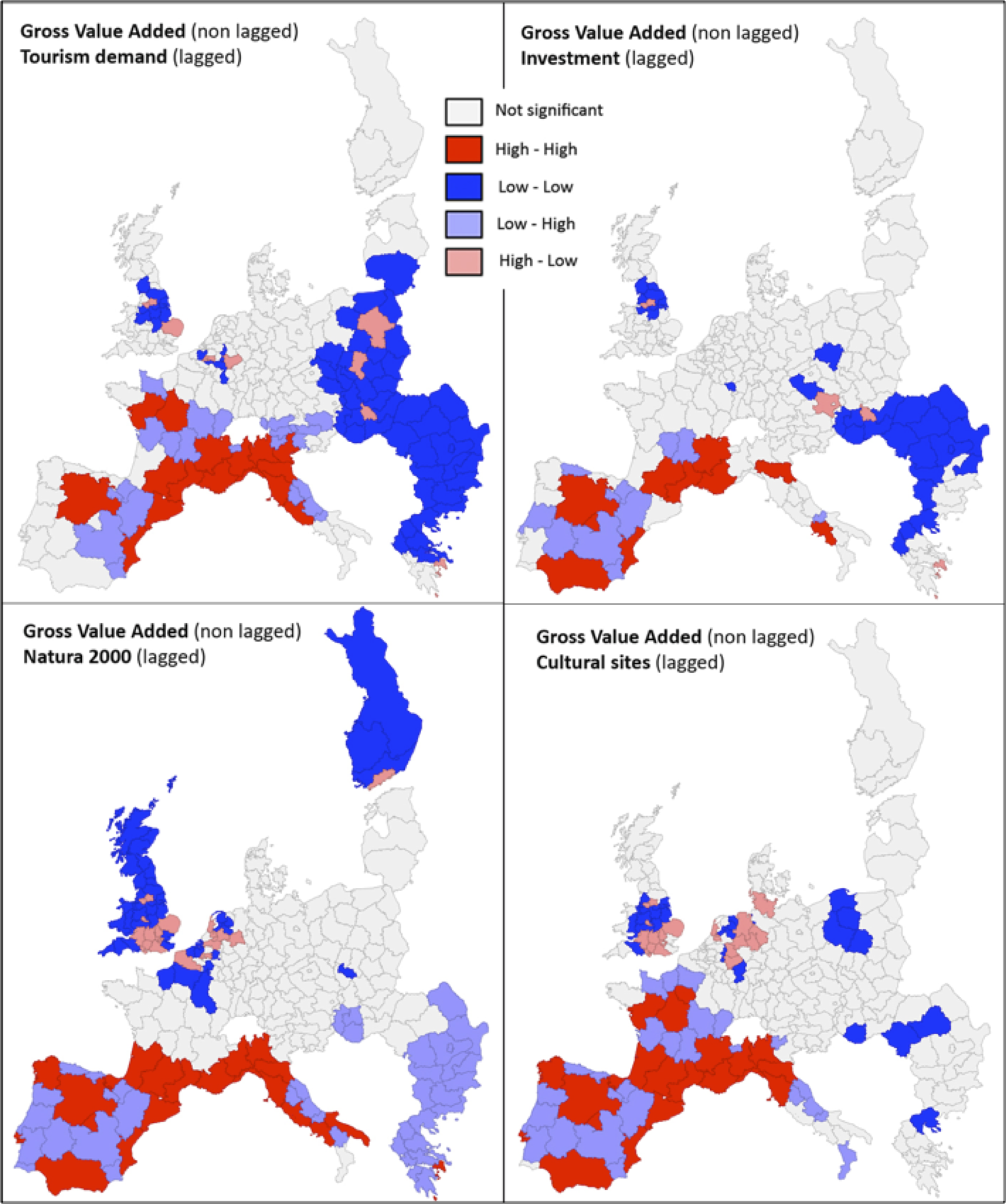
The first map (top-left) reveals a cluster of high values for tourism GVA and high tourism demand in southern western regions (dark red), while clusters of low values for both variables are located in the east side of Europe (dark blue). Nevertheless, the existence of a large number of southern regions (mostly in Spain, France and Italy) where low value added in tourism is spatially correlated with high tourism demand (light blue) is also noticeable, suggesting that tourism is possibly based on low value added products and services. A very similar pattern is observed for the second map (top-right), revealing that a large number of regions from Southern Europe (mostly concentrated in Spain) register high levels of investment in tourism while achieving relatively low levels of GVA.
The combination of these results (high tourism demand and high investments in the tourism sector) suggests a high mobilization of regional resources for tourism. However they generate a relatively low value added, which can be related to a low productivity in the utilization of these resources (nevertheless, it should be noted that this study does not address the specific question of productivity and does not provide a measure for the relation between the output of tourism activities and the necessary inputs for their provision). This tendency is even more marked when we observe the relation between GVA and natural resources (down-left) or cultural heritage (down-right). In the second case (cultural heritage), we can observe that for a large number of regions from Portugal, Spain, France and Italy low gross value added is correlated with a high number of cultural sites classified by UNESCO. On the other hand, when natural resources are taken into consideration, this tendency is also observable for Greek and Bulgarian regions (although it does not happen in France, suggesting that higher value added is achieved with nature oriented tourism in French regions).
Generally, these observations confirm the results obtained from the panel data model previously estimated: the negative correlation between natural resources and the GVA generated by tourism activities is not related to a low level of tourism demand in protected areas, but to the supply of massive, low value added tourism products and services in these regions. Even if some of them (located in coastal areas) register high levels of tourism GVA, a large number of territories (mostly those without direct connection to the sea) do not achieve good performance in terms of GVA despite the high tourism demand.
3.4 Spatial Econometric Analysis
The final step of this work is the computation of a spatial regression model by adding the spatial effects explicitly to the panel data model presented in (1). The existence of a spatially lagged endogenous variable (included as one more explanatory variable and capturing potential endogenous interaction effects) and spatial effects in the error term (a spatial multiplier that captures un-modelled spatial effects expressed in the interaction among the error terms) will be tested before estimation. In a general form, a space-time panel data model with spatial effects among the dependent variables and the error term can be specified as:

where
- Y it represents the log of tourism GVA in region i at time t.
- Xit corresponds to a 4x1 vector of independent variables for region i at time t,
namely:
- the number of nights in tourism establishments;
- the gross fixed capital formation in tourism;
- the percentage of the territory classified in Natura 2000;
- and the number of sites classified as World Heritage by UNESCO.
- W is a nonnegative N ×N matrix of known constants describing the spatial impacts; the element wij indicates the intensity of the relationship between cross sectional units i and j and the diagonal elements are set to zero because no region can be its own neighbour;
- WY represents the endogenous interaction effects among the dependent variables;
- Wu shows the interaction effects among the disturbance terms of the different units;
- ρ is the spatial autoregressive coefficient;
- λ the spatial autocorrelation coefficient;
- i is an index for the regions and t is an index for the time period.
The tests for the existence of spatial effects (Baltagi et al. 2003, 2007) were performed using the splm package in R (Milo, Piras 2012), aiming to identify whether the potential spatial effects are related to regional effects within the dependent variable (a spatial lag model, with λ = 0) and/or more general effects identified in the spatial distribution of the error terms (spatial error model, with ρ = 0). The score of 1469.973 obtained for the LM (Lagrange Multiplier) test implies the rejection of the null hypothesis of no random effects and no spatial autocorrelation (H0: λ = ρ = 0) and suggests the existence of spatial effects related to the dependent variable and/or the spatial correlation among the error terms (alternative hypothesis is that at least one component is not zero). In fact, the Moran I test computed in the previous section had already shown the existence of spatial effects (implying ρ≠0).
The Baltagi, Song and Koh’s SLM1 marginal test evaluates the inexistence of autoregressive spatial effects (H0: ρ = 0), assuming that no spatial effects exist in the error term (λ = 0); the score of 0.0187 with a p-value of 0.9851 implies non-rejection of the null hypothesis. Conversely, Baltagi, Song and Koh’s SLM2 marginal test, tests the null hypothesis of no spatial effects in the error term (H0: λ = 0) assuming no autoregressive spatial effects (ρ = 0); the score of 0.00847 with a p-value of 0.9933 also implies non-rejection of the null hypothesis. Thus, the inexistence of one type of spatial effects also implies the inexistence of the other. Finally, applying Baltagi, Song and Koh’s conditional test, LMλ, for no regional effects expressed in the error term (H0: λ = 0), independently of the value of ρ, a score of 37.1293 was obtained leading to the rejection of the null hypothesis. Thus, it is possible to conclude for the existence of spatial autocorrelation effects in the error term.
The existence of both types of spatial effects leads to the computation of a general spatial Cliff-Ord type model (Cliff, Ord 1981), including a spatially lagged dependent variable and a spatially autocorrelated error term. Finally, the results obtained for a spatial Hausmann test lead us to opt for a fixed effects model.
This spatial lag and spatial error model [with: Y =logGVA and X =(logNIT, log INV, NAT, HERIT)] is defined according to expression (2) previously presented, considering fixed individual effects and requiring a specification of the disturbances assuming that spatial autocorrelation applies to both the individual effects and the error term (with the transformation proposed by Kapoor et al. 2007, for the disturbance term following a first order spatial autoregressive process – “kkp” type). Table 3 presents the results obtained based on maximum likelihood estimation:
| Parameter | Estimate | Std.Error | t-value
| |||
| Intercept | -0. | 330*** | 0. | 028 | 3. | 843 |
| logNIT | 0. | 252*** | 0. | 014 | 17. | 787 |
| logINV | 0. | 655*** | 0. | 013 | 50. | 138 |
| NAT | -0. | 019*** | 0. | 001 | -14. | 940 |
| HERIT | -0. | 005 | 0. | 008 | -0. | 675 |
| Spatial autoregressive |
0.402*** | 0.040 | 10.067
| |||
| coefficient (ρ) | ||||||
| Spatial autocorrelation | 0.109*** |
0.028 |
3.843
| |||
| coefficient (λ) | ||||||
Although the computation of the R-square statistic is not possible in a spatial context, other results (also with important limitations, as discussed by Elhorst 2014) reveal a relevant increase in the adjustment regarding the model without spatial effects. The computation of a squared correlation coefficient between actual and fitted values (proposed by Elhorst 2014) has led to a result of 0.833 (0.320 for the model without spatial effects previously presented), while the computation of a Pseudo R-squared based on the quotient between the variance of the estimations and the variance of the actual values (proposed by Anselin, Lozano-Gracia 2008) has led to a result of 0.883 (0.830 for the model without spatial effects). Even if the measures of goodness of fit have important limitations in both cases, the model with spatial effects clearly performs better than the model without spatial effects.
Comparing the estimated parameters with those obtained from the model without spatial effects, the same type of relations (expressed in the sign of the correlations) between the dependent variable and the independent variables were identified although the impact of cultural assets loses statistical significance when spatial effects are included. This model confirms the expected positive correlation between tourism GVA, tourism demand and investment in the tourism sector, but in this case the impact of investment is higher than the impact of tourism demand. Possibly, a part of the regional dynamics (linked to tourism demand) is now captured by spatial effects associated to the lagged variable (tourism GVA), while the impact of cultural assets can eventually be captured by unmodelled spatial effects related to the error term. The model also confirms the negative correlation between regional natural resources and tourism GVA previously observed, which is the most important result arising from this analysis.
The existence of spatial effects among regions is also clear. The spatial effects identified in the space-time model reveal the existence of spillover effects (expressed in the positive value of the spatial autoregressive coefficient, showing that tourism dynamics in one region has positive consequences on the contiguous regions) and also unmodelled effects (expressed in the positive value of the spatial autocorrelation coefficient). Although it is clear that a major part of these effects are captured by the spatial distribution of the dependent variable (with a much larger estimated parameter), the existence of spatial effects in the distribution of the error terms suggests that other type of variables can be included in further works in order to increase the explanatory power of the model.
4 Discussion and Concluding Remarks
A first important conclusion of this study is the confirmation of the useful contribution of spatial analysis in tourism studies with a clear impact on the goodness of fit of the econometric model and the identification of spatial patterns in tourism activities and its determinants. It was possible to conclude from our exploratory spatial analysis that the impacts of the determinants of competitiveness taken into consideration differ across the territorial units despite the existence of a general trend identified by the econometric model. This is the first contribution of this work, leading from a policy point of view to the idea that the implementation of guidelines to improve tourism competitiveness must take into account the specific territorial conditions.
The results of this spatial analysis also imply that contemporary regional tourism dynamics is related, not only to regional resources and conditions, but also to the dynamics observed in neighbouring regions. This also has clear implications for tourism policies suggesting that local resource management, promotional strategies, transport systems or accommodation provision can be more efficiently planned if there is some collaboration among clusters of regions with similar characteristics. In fact, this type of complementarity between regions is possible to observe in many parts of Europe, even belonging to different countries as can be observed in e.g. mountain areas like the Alps (Switzerland and Italy) or the Pyrenees (Spain and France) or along major rivers (like the Danube).
The analysis of the determinants of regional competitiveness developed through the computation of a spatial panel data model confirmed the expected positive correlations between GVA generated by tourism activities, regional tourism demand and investment in the tourism sector. Nevertheless, the results also showed a negative relation between tourism GVA and the existence of natural resources. Although this negative correlation could be linked to the type of data used in the model (suggesting that it could be related to protective measures implemented in these areas), it was also possible to observe that regions with more protected areas are located in Southern European areas with high levels of tourism demand where mass tourism prevails.
A second contribution of this work for the existing literature is the identification of this negative correlation between the existence of rich natural resources and tourism competitiveness in European regions, which was only possible through the combined analysis of the econometric model (providing an overall general explanation) and the exploratory spatial analysis (identifying different spatial patterns and highlighting the role of Southern European territories in this context). In fact, the indicators of spatial autocorrelation used for the exploratory spatial analysis revealed the existence of a large number of regions from Southern Europe where abundant natural resources coexist with high levels of tourism demand and low value added in the tourism sector. Thus, the results suggest that massive tourism related to natural resources tends to generate less positive impacts on the regional GVA, despite its potential negative impacts on ecosystems and landscapes.
This analysis reveals an unsustainable process of tourism development for these regions apparently following a cost leadership competitive strategy based on low prices. Instead, taking into consideration their richness in terms of natural and cultural assets, a strategy of differentiation aiming at the provision of unique experiences based on the specific territorial resources could lead to a more sustainable form of tourism development. This would reinforce the linkage with other local economic activities with larger impacts on regional development and higher protection of sensitive resources. In fact, good practices related to this kind of utilization of natural resources for the creation of high value tourism products and services can already be found in many natural parks all over the world including Europe, while countries like Australia or New Zealand tend to give very high importance to these services within their tourism activities.
Finally, it is important to notice that the increasing amount of geo-referenced information related to tourism opens new opportunities for the application of spatial analysis techniques in order to identify spatial patterns of tourism development. Questions related to the effective usage of natural or cultural resources as tourism products or a more detailed analysis of tourism infrastructures can be integrated into similar models in the future, along with the consideration of other determinants of tourism competitiveness (marketing, management, planning, etc.). Another possible development of this work relates to the scale of analysis, given that NUTS 2 regions can include different tourism destinations within the same territory. The NUTS 3 level can be more appropriate for this purpose when comparable relevant statistical information is available.
References
Anselin L (2005) Exploring spatial data with GeoDaTM: A workbook. Center for Spatially Integrated Social Science, Santa Barbara http://la1.rcc.uchicago.edu/media/geoda_files/docs/geodaworkbook.pdf
Anselin L (2010) Thirty years of spatial econometrics. Papers in Regional Science 89: 3–25. CrossRef.
Anselin L, Lozano-Gracia N (2008) Errors in variables and spatial effects in hedonic house price models of ambient air quality. Empirical Economics 34: 5–34. CrossRef.
Baltagi S, Jung B, Koh W (2003) Testing panel data regression models with spatial error correlation. Journal of Econometrics 117: 123–150. CrossRef.
Baltagi S, Jung B, Koh W (2007) Testing for serial correlation, spatial autocorrelation and random effects using panel data. Journal of Econometrics 140[1]: 5–51. CrossRef.
Buhalis D (1999) Limits of tourism development in peripheral destinations: problems and challenges. Tourism Management 20: 183–185
Buhalis D (2000) Marketing the competitive destination of the future. Tourism Management 21: 97–116. CrossRef.
Butler R (1999) Sustainable tourism: A state-of-the-art review. Tourism Geographies 1[1]: 7–25. CrossRef.
Camisón C, Forés B (2015) Is tourism firm competitiveness driven by different internal or external specific factors? New empirical evidence from Spain. Tourism Management 48: 477–499
Celant A (2007) Global Tourism and Regional Competitiveness. Patron, Bologna
Clark T, Liner D (2015) Should I use fixed or random effects? Political Science Research and Methods 3[2]: 399–408. CrossRef.
Cliff A, Ord J (1981) Spatial Processes, Models and Applications. Pion, London
Cracolici M, Nijkamp P (2008) The attractiveness and competitiveness of tourist destinations: A study of southern Italian regions. Tourism Management 30: 336–344. CrossRef.
Croissant Y, Millo G (2008) Panel data econometrics in R: The plm package. Journal of Statistical Software 27[2]: 1–43. CrossRef.
Croissant Y, Millo G, Tappe K, Toomet O, Kleiber C, Zeileis A, Henningsen A, Andronic L, Schoenfelder N (2016) Package “plm”. CRAN, https://cran.r-project.org/web/packages/plm/plm.pdf
Cuccia T, Guccio G, Rizzo I (2016) The effects of UNESCO world heritage list inscription on tourism destinations performance in Italian regions. Economic Modelling 53: 494–508. CrossRef.
Cucculelli M, Goffi G (2016) Does sustainability enhance tourism destination competitiveness? Evidence from Italian destinations of excellence. Journal of Cleaner Production 111: 370–382. CrossRef.
Elhorst J (2003) Specification and estimation of spatial panel data models. International Regional Science Review 26: 223–243. CrossRef.
Elhorst J (2014) Spatial Econometrics: From Cross-Sectional Data to Spatial Panels. Springer, New York
European Commission (2007) Agenda for a sustainable and competitive European tourism. European Commission, Luxembourg. http://eur-lex.europa.eu/legal-content/EN/TXT/?uri=celex:52007DC0621
Florax R, Vlist A (2003) Spatial econometric data analysis: Moving beyond traditional models. International Regional Science Review 26[3]: 23–243. CrossRef.
Hassan S (2000) Determinants of market competitiveness in an environmentally sustainable tourism industry. Journal of Travel Research 38[3]: 239–245. CrossRef.
Jafari J (2001) The scientification of tourism. In: Smith V, Brent M (eds), Hosts and Guests Revisited: Tourism Issues of the 21st Century. Cognizant Communication Corporation, New York
Kang S, Kim J, Nicholls S (2014) National tourism policy and spatial patterns of domestic tourism in South Korea. Journal of Travel Research 53[6]: 791–804. CrossRef.
Kapoor M, Kelejian HH, Prucha IR (2007) Panel data model with spatially correlated error components. Journal of Econometrics 140[1]: 97–130. CrossRef.
Kozak M (1999) Destination competitiveness measurement: Analysis of effective factors and indicators. European Regional Science Association Conference Papers, Dublin, http://www-sre.wu-wien.ac.at/ersa/ersaconfs/ersa99/Papers/a289.pdf
Ma T, Hong T, Zhang H (2015) Tourism spatial spillover effects and urban economic growth. Journal of Business Research 68[1]: 74–80. CrossRef.
Majewska J (2015) Inter-regional agglomeration effects in tourism in Poland. Tourism Geographies 17[3]: 408–436. CrossRef.
Marrocu E, Paci R (2013) Different tourists to different destinations – evidence from spatial interaction models. Tourism Management 39: 71–83. CrossRef.
Martín J, Mendoza C, Román C (2017) A DEA travel-tourism competitiveness index. Social Indicators Research 130[3]: 1–21. CrossRef.
Mazanek J, Wober K, Zins A (2007) Tourism destination competitiveness: From definition to explanation? Journal of Travel Research 46: 86–95. CrossRef.
Milo G, Piras G (2012) splm: Spatial panel data models in R. Journal of Statistical Software 47[1]: 1–38. CrossRef.
Navickas V, Malakauskaite A (2009) The possibilities for the identification and evaluation of tourism sector competitiveness factors. Engineering Economic 1[61]: 37–44
O’Brien R (2007) A caution regarding rules of thumb for variance inflation factors. Quality and Quantity 41[5]: 673–690. CrossRef.
Park J, Jang S (2014) An extended gravity model: Applying destination competitiveness. Journal of Travel & Tourism Marketing 31[7]: 799–816
Patuelli R, Mussoni M, Candela G (2013) The effects of world heritage sites on domestic tourism: A spatial interaction model for Italy. Journal of Geographical Systems 15: 369–402. CrossRef.
Pesaran MH (2007) A simple panel unit root test in the presence of cross-section dependence. Journal of Applied Econometrics 22[2]: 265–312. CrossRef.
Pesaran MH, Ullah A, Yamagata T (2008) A bias-adjusted LM test of error cross-section independence. The Econometrics Journal 11[1]: 105–127. CrossRef.
Poon A (1994) The ‘new tourism’ revolution. Tourism Management 15[2]: 91–92. CrossRef.
Porter M (1985) Competitive advantage – creating and sustaining superior performance. The Free Press, New York
Porter M (2003) The economic performance of regions. Regional Studies 37[6/7]: 549–578. CrossRef.
Ritchie J, Crouch G (2003) The competitive destination: A sustainable tourism perspective. CABI International, Oxfordshire. CrossRef.
Romão J (2015) Culture or nature: A space-time analysis on the determinants of tourism demand in European regions. Discussion papers spatial and organisational dynamics 14, http://www.cieo.pt/discussionpapers/discussionpapers14.pdf, Research Centre for Spatial and Organizational Dynamics, Faro
Sharpley R (2009) Tourism Development and the Environment: Beyond Sustainability? London
Song H, Dwyer L, Cao Z (2012) Tourism economics research: A review and assessment. Annals of Tourism Research 39[3]: 1653–1682. CrossRef.
Tsai H, Song H, Wong K (2009) Tourism and hotel competitiveness. Journal of Travel and Tourism Marketing 26[5]: 522–546. CrossRef.
UNESCO (2000) Sustainable Tourism and the Environment. UNESCO, Paris
UNESCO (2005) World Heritage Centre – Sustainable Tourism Programme. UNESCO, Paris
UNWTO (2007) Practical Guide to Tourism Destination Management. UNWTO, Madrid
Vanhove N (2005) The Economics of Tourism Destinations. Elsevier, Oxford. CrossRef.
Wall G, Mathieson A (2006) Tourism: Change, Impacts and Opportunities. Pearson, Essex
Weaver D (2006) Sustainable tourism: Theory and practice. Elsevier, Oxford. CrossRef.
Webster C, Ivanov S (2014) Transforming competitiveness into economic benefits: Does tourism stimulate economic growth in more competitive destinations? Tourism Management 40: 137–140. CrossRef.
Williams P, Ponsford I (2009) Confronting tourism’s environmental paradox: Transitioning for sustainable tourism. Futures 41: 396–404. CrossRef.
World Commission on Environment and Development (1987) Our Common Future. Oxford University Press, New York
World Economic Forum (2008) The Travel and Tourism Competitiveness Report 2008. World Economic Forum, Geneva
Yang Y, Fik T (2014) Spatial effects in regional tourism growth. Annals of Tourism Research 46: 144–162. CrossRef.
A Appendix
| Fixed Effects | Random effects | Pooling effects
| ||||
| Est. | Est. | Est.
| ||||
| Intercept | 2. | 978*** | 0. | 686*** | ||
| NAT | -0. | 003* | -0. | 007*** | -0. | 021*** |
| HERIT | 0. | 031* | 0. | 062 | 0. | 003 |
| logINV | 0. | 049*** | 0. | 130*** | 0. | 686*** |
| logNIG | 0. | 146*** | 0. | 316*** | 0. | 236*** |
| Adj. R2 | -0. | 090 | 0. | 236 | 0. | 802 |
In this case, logarithms were applied to the variables Tourism Gross Value Added (dependent variable), Gross Fixed Capital Formation in tourism (logINV) and nights spent in tourism accommodation establishments (logNIG).
| Fixed Effects | Random effects | Pooling effects
| ||||
| Est. | Est. | Est.
| ||||
| Intercept | 4180. | 750*** | 2800. | 108*** | ||
| NAT | -1. | 094 | -6. | 397 | -83. | 236*** |
| HERIT | 25. | 354 | 69. | 189 | 62. | 367 |
| INVpc | 0. | 071 | 0. | 196*** | 3. | 677*** |
| NIGpc | 100. | 813*** | 127. | 257*** | 61. | 196*** |
| Adj. R2 | -0. | 120 | 0. | 052 | 0. | 553 |
In this case, the values for the variables Tourism Gross Value Added (dependent variable), Gross Fixed Capital Formation in tourism (INVpc), and nights spent in tourism accommodation establishments (NIGpc), were divided by the number of residents (per capita), in order to consider the dimension of the regions. Nevertheless, the results obtained were much less significant.