 Volume
3, Number 2, 2016, 47–60 journal homepage:
region.ersa.org
Volume
3, Number 2, 2016, 47–60 journal homepage:
region.ersa.orgDOI: 10.18335/region.v3i2.129
Cities and Inequality*
1 University of Milan-Bicocca, Milan, Italy (email: alessandra.michelangeli@unimib.it)2 University of Verona, Verona, Italy (email: eugenio.peluso@univr.it)
*Financial support by the Italian Ministry of University and Research is gratefully acknowledged. The authors gratefully acknowledge the Osservatorio del Mercato Immobiliare for housing market data; the Fondazione Rodolfo De Benedetti for labour market data; and Istituto Tagliacarne for data about local amenities. An earlier version of the paper was presented at the 55th ERSA Congress in Lisbon. We would like to thank the participants at this conference for their useful comments. We thank the editor Paolo Veneri and two anonymous reviewers for their constructive comments. The usual disclaimer applies.
Abstract. We propose an innovative methodology to measure inequality between cities. If an even distribution of amenities across cities is assumed to increase the average well-being in a given country, inequality between cities can be evaluated through a multidimensional index of the Atkinson (1970) type. This index is shown to be decomposable into the sum of inequality indices computed on the marginal distributions of the amenities across cities, plus a residual term accounting for their correlation. We apply this methodology to assess inequality between Italian cities in terms of the distribution of public infrastructures, local services, economic and environmental conditions.
JEL classification: R11, R12, R23
Key words: Inequality, inequality aversion, social welfare, city
1 Introduction
Recent literature has shown that excessive inequality produces negative effects not only for disadvantaged individuals but also for a whole community. The State of the World’s Cities Report by UN-Habitat (2008) established an international alert line corresponding to a Gini coefficient1 value of 0.4. Several African and Latin American cities exhibit a value of Gini coefficient above this threshold2 . High income inequality can have drastic consequences of economic, social, and political nature, such as lack of investment, protests and riots, and civil conflicts. In addition, high inequality may lead to the weak functioning of labor markets, inadequate investments in public services, or institutional and structural failures in income redistribution (UN-Habitat 2008)3 . Given the importance of having an even distribution of resources, or at most moderate levels of inequality, to the normal functioning of a community, in this paper we focus on inequality across cities because we are witnessing a dramatic increase of people living in urban areas over the last 60 years. According to United Nations and World Health Organization projections, while less than one-third of the world’s population lived in cities in 1950, about two thirds of humanity is expected to live in urban areas by 2030 (UN-Habitat 2008, WHO-UN Habitat 2016). Local facilities and public goods available at the city-level may have an impact on individual well-being. As a result, there has been a growing interest on complementing income measures with the value of public goods and services that are available at the municipality, provincial, or regional level (Aaberge et al. 2010). Following a multidimensional approach, we consider inequality in terms of urban disparities, i.e. provincial capitals rather than in terms of differences across individuals. We propose an innovative methodology, which relies on the assumption that an even distribution of local goods and services across cities increases the average level of well-being in a given country. Due to the spatial nature of such goods and services, not all individuals in a society are equally exposed to the same quantities and qualities of them. Location choices are also driven by preferences for local public goods so even though these goods are not marketable, their impact on individual utility is capitalized in housing and labor markets. The hedonic approach is used to obtain a monetary evaluation of local public goods, named amenities, and defined as location specific characteristics with positive or negative effects on household’s utility (Bartik, Smith 1987). People living in different cities face different amenities, and this generates inequalities across individuals in the level of welfare they locally perceive. The link between welfare and inequality in a multidimensional setting is captured by the Abul Naga, Geoffard (2006) index. We extend their methodology by endogenously determining the parameters of the index through a hedonic model referred to the housing and labor markets.
We employ our methodology to assess inequality between 103 Italian provincial (NUTS-3) capitals on the basis of a set of localized goods, such as public infrastructure, local services, economic, and environmental conditions. The proposed methodology allows to disentangle not only the effect of the distribution of each amenity on overall inequality, but also the effect of the joint distribution of amenities in determining overall inequality across cities.
The multidimensional inequality index turns out to display a value indicating that there are significant disparities between cities, mainly due to differences in the availability of services and infrastructure, in particular health services, economic conditions, transport infrastructure, and educational services. Environmental conditions and cultural amenities play a minor role in determining the overall level of inequality.
The paper is organized as follows. In Section 2 we present the theoretical framework by deriving the multidimensional inequality index from a social evaluation function having specific properties. Section 3 describes the data. Section 4 presents the results. Section 5 concludes the paper.
2 Framework
This section first shows how to obtain the multidimensional inequality index (Section 2.1). Then the Rosen (1979) and Roback (1982) model is briefly reviewed to show how implicit prices of amenities are determined (Section 2.2). Implicit prices are needed to endogenously determine the value of the multidimensional inequality index parameters.
2.1 Assessing multidimensional inequality
To derive the multidimensional inequality index, we proceed in two steps. First, we introduce a function measuring the level of well-being in a given city, provided by a bundle of k amenities4 . Second, we aggregate the levels of well-being specific to each city in the simplest way, i.e. by considering their mean.
Let us consider n cities, indexed by i = 1,…,n. Each city is endowed with k amenities,
which are all strictly positive. The quantities owned by city i are denoted by the vector
 i = (zi1,…,zij,…,zik) ∈ R++k.
We assume that an increasing and concave function w( i) measures the social evaluation of
well-being in city i, as a function of the available amenities, and we define the average
evaluation function among the n cities as W(
i) measures the social evaluation of
well-being in city i, as a function of the available amenities, and we define the average
evaluation function among the n cities as W( 1,…
1,… n) =
n) =  ∑
i=1nw(
∑
i=1nw( i). The monotonicity of
w(⋅) implies that an increase in the quantity of any amenity in any city results to be socially
desirable. The concavity of w(⋅) implies inequality aversion, that is, it would be socially
desirable having a homogeneous level of amenities across cities, rather than cities exhibiting
huge disparities in terms of public goods, services, and infrastructure. Under the assumption of
inequality aversion, society is willing to renounce a share of amenities to obtain an equitable
distribution of them across cities. The higher inequality aversion, the higher the share society
is willing to renounce. This idea was initially introduced in the risk literature by
Pratt (1964) through the concept of “certainty equivalent”, which is the amount of money a
decision maker is willing to pay to undertake a risky decision. It is a function of the
risk attitude of the decision maker. Atkinson (1970) imported in inequality and
welfare measurement the notion of certainty equivalent by defining the analogous
concept of “equally distributed equivalent income”, which is the amount of income
that, if equally distributed across individuals, would enable the society to reach the
same level of welfare as the actual (unequal) distribution of incomes. The equally
distributed equivalent income has been extended to the multidimensional case by
Tsui (1995, 1999) (see also Gajdos, Weymark 2005, Abul Naga, Geoffard 2006;
Weymark 2006 for a survey). In this paper, we transpose these concepts in comparing
well-being among cities. More precisely, we define the vector of equally distributed
equivalent amenities as the quantity of amenities that, if equally distributed across the
n cities, guarantee the same average well-being as the (unequal) current amenity
distribution.
i). The monotonicity of
w(⋅) implies that an increase in the quantity of any amenity in any city results to be socially
desirable. The concavity of w(⋅) implies inequality aversion, that is, it would be socially
desirable having a homogeneous level of amenities across cities, rather than cities exhibiting
huge disparities in terms of public goods, services, and infrastructure. Under the assumption of
inequality aversion, society is willing to renounce a share of amenities to obtain an equitable
distribution of them across cities. The higher inequality aversion, the higher the share society
is willing to renounce. This idea was initially introduced in the risk literature by
Pratt (1964) through the concept of “certainty equivalent”, which is the amount of money a
decision maker is willing to pay to undertake a risky decision. It is a function of the
risk attitude of the decision maker. Atkinson (1970) imported in inequality and
welfare measurement the notion of certainty equivalent by defining the analogous
concept of “equally distributed equivalent income”, which is the amount of income
that, if equally distributed across individuals, would enable the society to reach the
same level of welfare as the actual (unequal) distribution of incomes. The equally
distributed equivalent income has been extended to the multidimensional case by
Tsui (1995, 1999) (see also Gajdos, Weymark 2005, Abul Naga, Geoffard 2006;
Weymark 2006 for a survey). In this paper, we transpose these concepts in comparing
well-being among cities. More precisely, we define the vector of equally distributed
equivalent amenities as the quantity of amenities that, if equally distributed across the
n cities, guarantee the same average well-being as the (unequal) current amenity
distribution.
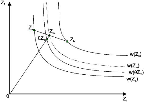
Figure 1 shows the simple case with two cities: a and b, and two amenities: z1 and z2. We assume cities a and b are endowed with the bundles Za = (Z1a,Z2a) and Zb = (Z1b,Z2b), respectively. The distribution of two amenities is unequal since city a has a greater quantity of amenity 2 and a lower quantity of amenity 1, compared with city b.
Let us define Zm = (Z1m,Z2m) the mean bundle, containing the average quantity of each amenity, that is Z1m = (Z1a + Z1b)∕2 and Z2m = (Z2a + Z2b)∕2.
Jensen’s inequality5 implies that the level of social well-being would be higher if a and b were endowed with the same bundle of amenities Zm rather than with their actual bundles Za and Zb. In formal terms,
 | (1) |
By continuity and monotonicity of W(⋅), starting from (1) it is possible to find a positive scaling factor θ < 1, such that the bundle θZm = (θZ1m,θZ2m) satisfies 2W(θZm) = W(Za) + W(Zb). The vector θZm contains the equally distributed equivalent amenities mentioned above, which guarantee the same average level of well-being provided by the actual (unequal) amenity distribution across cities.
Abul Naga, Geoffard (2006) provide an axiomatic characterization of θ as an index of
relative equality and its complement to one (1 - θ) as a (relative) index of inequality. While
a formal presentation of their framework goes beyond the scope of this paper, we
point out the assumptions needed to formulate the multidimensional inequality index
(1 - θ), such that it can be used to measure inequality between cities. The social
evaluation function is assumed to take a Cobb-Douglas form, w( i) = ∏
j=1kzijσj. The
parameter σj captures the aversion to an unequal distribution of amenity - across
cities. In Section 2.1 we further discuss the role of this parameter in the setup and
present the methodological strategy to determine the value of σ associated with each
amenity.
i) = ∏
j=1kzijσj. The
parameter σj captures the aversion to an unequal distribution of amenity - across
cities. In Section 2.1 we further discuss the role of this parameter in the setup and
present the methodological strategy to determine the value of σ associated with each
amenity.
The equality index θ has been shown to be decomposable into k indexes, one for amenity, related to the marginal distribution of amenities, and a residual term based on the dependence structure between amenities. In formal terms,
 | (2) |
where γj, with j01,…,k are k unidimensional indices of the Atkinson (1970)
type, i.e. γj = 
![[1∑n σj]
n i=1zij](12916x.png)
 ; ρ is an interaction term equal
to6
ρ =
; ρ is an interaction term equal
to6
ρ = 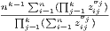 .
.
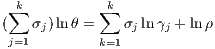
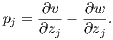
The complement to 1 of γj, i.e. 1 - γj, is the Atkinson index of inequality for amenity j. Notice that the value of parameters σj determines not only the degree of inequality aversion in the evaluation function w(⋅), but also the weight assigned to amenity j in the θ decomposition (1). In multidimensional inequality literature, equal weights are usually assumed for the different attributes under exam, as in the Human Development Index, as well as in studies by other institutions and scholars such as Becker et al. (2005) and Croci Angelini, Michelangeli (2012). In this paper, we follow Brambilla et al. (2013) to endogenously determine the values of σj. They are set to their respective weight on the monetary assessment of the amenity bundle with sample average quantities. The monetary value of amenities, denoted by pj, with j = 1,…,k, is determined on the basis of hedonic regressions based on the housing prices individuals are willing to pay and the wages they are willing to accept to locate in a given city. More precisely, σj, with j = 1,…,k, is defined as:
 | (3) |
where
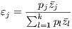 | (4) |
Each parameter εj is set to be equal to the ratio between the estimated value of the average quantity of the amenity j and the value of all amenities. The methodology implicitly assumes that the higher the contribution of amenity j in determining the amenity bundle value, the more intense is the aversion for its uneven distribution across cities, the lower will be the value of σj.
In the next section, we determine the implicit prices of amenities, pj, by referring to the hedonic spatial equilibrium model, developed by Rosen (1979) and Roback (1982), which explain the optimal location choice of agents, i.e. consumers and firms.
It is worth mentioning that implicit or shadow prices of amenities could be computed using alternative approaches. For example, Veneri, Murtin (2016), in order to compute multidimensional living standards among OECD regions, use the life satisfaction approach to estimate the shadow price of three dimensions of well-being: income, jobs, and health outcomes.
2.2 Determining the implicit value of amenities
Rosen (1979) considers household and business location decisions in order to maximize utility and to minimize costs, respectively. Household choices depend on the wage that one can earn living in a given city and the cost of living approximated by the cost of housing services. Households with a preference for amenity-rich cities will move to those cities, which are also the more expensive, and will be willing to earn lower wages to enjoy the higher (lower) level of amenities (disamenities). Conversely, household living in low-amenity cities will be compensated with higher wages and lower housing prices. In equilibrium, no-one has an incentive to move, since the relocation costs are higher than the utility gains generated by moving. The representative household experiences the same level of utility in all cities, and unit production costs are equal to the unit production price. Roback (1982) extends the model in a general equilibrium setting, by considering the housing market in addition to the labor market, since the two markets are interconnected and both contribute to determine the implicit price of amenities. The implicit price is given by the sum of the housing price differential and the negative of the wage price differential.
The model is empirically implemented by estimating two separate equations for the log of housing prices and wages:

where vhit is the real price of housing unit h in city i at time t; Xhit is a vector of housing characteristics; Zit is a vector of amenities in city i; wmit is the real wage of individual m in city i at time t; Y mit is a vector of individual characteristics; ηhit ~ N(0;ση2) and ζmit ~ N(0;σζ2).
The implicit price of amenity zj is given by
 | (7) |
3 Data
We use our methodology to assess inequality between 103 provincial capitals observed in the period 2001-2010. We consider six amenities: cultural infrastructure, educational and health services, transport infrastructure; economic and environmental conditions (Table A.1 in the Appendix sets out the list of amenities with their sources). Cultural conditions, educational services and health services are measured each by an index provided by GuglielmoTagliacarne Institute at the provincial level in 2004. These three indices are used as proxy for services at the city-level. Each of these indices is set to 100 for the Italian average. Cultural conditions are measured by an index of cultural infrastructure accounting for museums, theatres, cinemas, libraries, gyms. The index for educational services combines information about the number of schools of all levels, public and private; the number of classrooms per school; presence of building facilities, such as recreation and gym facilities, library and computer lab facilities; the number of teachers. The index for health services aggregates statistical information about the number of doctors at all levels, the number of nurses and other auxiliary personnel, the number of hospital beds, and the number and types of medical devices. Transport infrastructure is measured by a multimodal index that considers accessibility by air, train and car. The index is at the city level and is set equal to 100 for the European average. It is provided for the year 2006 by European Observation Network for Territorial Development and Cohesion (ESPON) project. The employment rate serves as proxy for economic conditions. The rate is at the city level for the year 2010, and it is provided by the Italian National Institute of Statistics (ISTAT). Environmental conditions are represented by the air quality in terms of reduced number of polluting agents in the air. The variable for air quality was constructed setting the maximum number of air-polluting observed in our sample equal to zero and associating increasing integer values with the decreasing number of air-polluting agents. The numbers of polluting agents are at the city level, refer to 2004 and were from ISTAT. Table 1 presents summary statistics of amenity variables.
| Variable | Mean | Std. Dev. | Min. | Max. | Unit of | Year |
| observation | ||||||
| Cultural | 126.11 | 71.89 | 18.90 | 504.17 | Province | 2004 |
| infrastructure | ||||||
| Educational | 113.47 | 41.34 | 24.06 | 325.32 | Province | 2004 |
| services | ||||||
| Health services | 121.75 | 56.90 | 26.59 | 287.19 | Province | 2004 |
| Transport | 105.29 | 26.88 | 47.00 | 161.00 | Municipality | 2006 |
| Employment rate | 90.33 | 7.39 | 68.61 | 97.23 | Municipality | 2010 |
| Air quality | 9.96 | 3.12 | 0.00 | 18.00 | Municipality | 2004 |
The 103 provincial capitals of our sample have on average a higher endowment of cultural infrastructure, followed by health and educational services. The indicator for cultural infrastructure shows the largest variability, according the standard deviation, followed by health and educational services.
For the housing and labor markets, we use the same data set of Colombo et al. (2014) used to measure quality of life in the 103 cities. Housing market data are from the Real Estate Observatory of the Italian Ministry of Finance, and refer to individual house transactions in the 103 Italian provincial capitals between 2004 and 2010. In addition to sale prices, the dataset provides a detailed description of housing characteristics, such as total floor area, number of bathrooms, floor level, number of garages, location (center, semi center, suburb), and location (center, semi-center, suburbs).
Labor market data are from the Italian National Social Security Institute (INPS) for years 2001 and 2002 and were provided by Fondazione Rodolfo De Benedetti. The dataset provides information on the private sector employees’ annual earnings, the level of occupation, whether the job is full-time or part-time, contract length, province of work, and sector of economic activity. Personal and demographic characteristics include gender, age, nationality, and province of residence. Housing prices and wages are measured at constant 2004 prices. As mentioned in Colombo et al. (2014), the difference in the timing of the data between wages and housing prices is due to data availability. However considering that we are using only data on dependent employment (entrepreneurs and self-employed are not included) the cross-sectional variation across cities is relatively stable over time, and the actualization procedure applied to the data should account for the possible concerns on this issue7 .
4 Results
Equations (5) and (6) are estimated by OLS and the results are reported in Table A.1 and A.2, respectively, in the Appendix. Robust standard errors are used with clustering at city level in order to allow for within-city correlation. The covariates used in model (5) account for about 72 per cent of the variance of the logarithm of housing prices, while the marginal explanatory power of local amenities is about 7%. Model (6) explains 61 per cent of the variability of the logarithm of wages, while the marginal explanatory power of local amenities is about 1.8%. The amenity coefficients are jointly statistically significant in the two models (F = 15.01, p <0.00 for the housing price equation; F = 37.46, p <0.00 for the wage equation).
Full implicit prices for local amenities are shown in Table 2, column 2. The implicit price of amenity zj is given by (7). To calculate the first derivative, the estimated expected housing price and wage are obtained by (5) and (6), respectively. However, since the empirical specification for the housing price regression and wage regression are log-linear, the relation between the normal and the lognormal distribution has to be taken into account to derive appropriate estimates. The following results from the normal distribution are used. If Y is a normally distributed random variable with expected value μ and variance σ2, P = exp(Y ) is lognormally distributed with expected value equal to exp(μ + σ2∕2). Hence, the expected values of housing price and wages have been obtained by plugging in the estimated values in the previous formulas.
The implicit price of a given amenity can be interpreted as the monetary amount, expressed in Euro at constant 2004 prices, households would be willing to pay annually for a one-standard deviation change in that amenity. Increasing the index for educational services by one-standard deviation is valued €122, while the implicit prices associated with health services and cultural infrastructure are €91 and €7, respectively. The weakness of the influence of culture on housing and labor markets is common in hedonic studies on Milan and other Italian cities (for instance Colombo et al. 2014, Brambilla et al. 2013). This is a puzzling result demanding a deeper investigation. The estimated marginal willingness to pay for increasing the employment rate by one-standard deviation is €68. Increasing the ESPON index for transport infrastructure by one-standard deviation is valued €76. A marginal improvement in air quality is valued €21.
| Variable | Hedonic | Parameter measuring | Univariate |
| price* | inequality aversion** | inequality index | |
| pj | σj | 1 - γj | |
| Cultural infrastructure | 7 | 0.1956 | 0.4104 |
| Education | 122 | 0.1310 | 0.2482 |
| Health services | 91 | 0.1448 | 0.3270 |
| Transport | 76 | 0.1601 | 0.2560 |
| Employment rate | 68 | 0.1694 | 0.2783 |
| Air quality | 21 | 0.1989 | 0.2309 |
| Interaction term | |||
ρ =  | 1.3860
| ||
| Multidimensional | | ||
| Inequality Index | 0.3121
| ||
| I = 1 - θ | |||
**Higher values of σj imply lower levels of inequality aversion.
The amenity estimated implicit prices and the city average quantities are used to estimate
the vector of parameters  = (σ1,…,σk) according to equations (5) and (6). We recall that their
values, reported in Table 2, column 3, determine the level of inequality aversion and the weight
of each amenity in the θ decomposition, given by equation (2). The higher σj, with
j = 1,…,k, the lower aversion to an unequal distribution of amenity j across cities,
and the lower the value of the unidimensional inequality index for this amenity ,
i.e. 1 - γj. The highest degree of inequality aversion is for educational and health
services, followed by transport infrastructure and economic conditions, represented
by the employment rate. Inequality aversion is lower for air quality and cultural
amenities.
= (σ1,…,σk) according to equations (5) and (6). We recall that their
values, reported in Table 2, column 3, determine the level of inequality aversion and the weight
of each amenity in the θ decomposition, given by equation (2). The higher σj, with
j = 1,…,k, the lower aversion to an unequal distribution of amenity j across cities,
and the lower the value of the unidimensional inequality index for this amenity ,
i.e. 1 - γj. The highest degree of inequality aversion is for educational and health
services, followed by transport infrastructure and economic conditions, represented
by the employment rate. Inequality aversion is lower for air quality and cultural
amenities.
The last column of Table 2 shows the unidimensional inequality index of the Atkinson (1970) type, 1 - γj. It is lower for air quality and becomes progressively higher for educational services, transport infrastructure, employment rate, health services and cultural infrastructure.
As mentioned in Section 2, ρ measures the effect on inequality due to the interdependence relationship between amenities. If ρ equals one, there is no joint effect of amenities on the multidimensional inequality index; if ρ is less than 1, the joint effects tend to magnify, while if ρ is more than 1, they offset each other. Table 2 shows a value for ρ higher than 1 implying that the joint effect of amenities contributes to the decrease of inequality across cities.
Finally, the multidimensional inequality index (3) turns out to be equal to 0.3121.
To sum up, overall inequality is mainly due to educational and health services, transport infrastructure, and economic conditions because of the higher inequality aversion and the higher value of the unidimensional inequality index for the variables associated with these four amenities. Air quality and cultural infrastructure play a minor role in determining the overall degree of inequality either because the unidimensional inequality index and the degree of inequality aversion are low, as for air quality, or because the inequality aversion and the weight of the variable are low, as for cultural amenities.
We use the estimated values for  = (σ1,…,σk) to calculate the values of the
evaluation function W =
= (σ1,…,σk) to calculate the values of the
evaluation function W =  ∏
j=1kzijσj specified in Section 2, which gives the level of
well-being individuals enjoy from the endowment of the six amenities specific to each city.
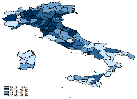
Table 3 reports the city-ranking for the value function W, and Figure 2 shows the
geographic distribution of W values across Italian cities. Looking at the map, a clear
North-South divide can be observed. A clustering of high scores can be observed for
cities in the Lombardy and Veneto regions. Cities in the South generally display
relatively lower values of W, with clustering of low scores in the cities of Molise,
Sardinia and Basilicata. Looking at the city size, well-being is generally higher in
large cities (Rome, Milan, Naples) or medium-sized cities (Trieste, Firenze, Padua,
Pisa).
∏
j=1kzijσj specified in Section 2, which gives the level of
well-being individuals enjoy from the endowment of the six amenities specific to each city.
Table 3 reports the city-ranking for the value function W, and Figure 2 shows the
geographic distribution of W values across Italian cities. Looking at the map, a clear
North-South divide can be observed. A clustering of high scores can be observed for
cities in the Lombardy and Veneto regions. Cities in the South generally display
relatively lower values of W, with clustering of low scores in the cities of Molise,
Sardinia and Basilicata. Looking at the city size, well-being is generally higher in
large cities (Rome, Milan, Naples) or medium-sized cities (Trieste, Firenze, Padua,
Pisa).
| City | W | City | W | City | W | City | W |
| Trieste | 103.65 | Forli | 62.62 | Biella | 54.62 | Asti | 47.96 |
| Firenze | 97.28 | Vicenza | 62.58 | Ascoli Piceno | 54.57 | Reggio Calabria | 47.33 |
| Roma | 88.56 | Brescia | 61.95 | Rovigo | 54.08 | Cosenza | 46.81 |
| Milano | 85.48 | Pistoia | 61.59 | Chieti | 53.90 | Vibo Valentia | 45.56 |
| Padova | 81.92 | Bari | 61.17 | Palermo | 53.68 | Sassari | 45.51 |
| Pisa | 81.35 | Novara | 60.82 | Viterbo | 53.40 | Ragusa | 45.29 |
| Napoli | 80.36 | Verona | 60.43 | Lecce | 53.36 | Cuneo | 44.84 |
| Varese | 76.02 | Livorno | 60.20 | Pescara | 53.13 | Trapani | 44.41 |
| Pavia | 74.84 | Prato | 59.84 | Cagliari | 52.88 | Campobasso | 43.31 |
| Bologna | 73.20 | Imperia | 59.73 | Caserta | 52.49 | Vercelli | 43.01 |
| Gorizia | 72.88 | La Spezia | 59.62 | Latina | 52.09 | Taranto | 42.91 |
| Lucca | 70.29 | Savona | 59.41 | Benevento | 52.05 | Isernia | 42.23 |
| Rimini | 69.62 | Massa | 59.24 | Udine | 51.47 | Oristano | 41.93 |
| Ancona | 69.41 | Catania | 58.44 | Pordenone | 50.71 | Aosta | 41.80 |
| Venezia | 69.06 | Ravenna | 58.30 | Alessandria | 50.54 | Siracusa | 41.75 |
| Torino | 69.01 | Mantova | 58.25 | Verbania | 50.35 | Potenza | 41.17 |
| Cremona | 68.79 | Ferrara | 57.58 | Trento | 50.20 | Rieti | 40.41 |
| Modena | 68.22 | Avellino | 57.38 | Bolzano | 49.97 | Foggia | 39.05 |
| Bergamo | 67.01 | Frosinone | 57.29 | Piacenza | 49.73 | Agrigento | 37.24 |
| Como | 66.23 | Treviso | 56.68 | Belluno | 49.61 | Crotone | 36.50 |
| Macerata | 65.57 | Siena | 56.67 | Teramo | 49.35 | Caltanissetta | 36.19 |
| Lecco | 65.13 | Salerno | 56.45 | Catanzaro | 49.00 | Grosseto | 36.11 |
| Genova | 64.70 | Messina | 55.63 | Sondrio | 48.79 | Enna | 35.34 |
| Lodi | 63.88 | L’Aquila | 55.19 | Arezzo | 48.30 | Matera | 33.10 |
| Parma | 63.17 | Reggio Emilia | 54.80 | Terni | 48.23 | Nuoro | 30.95 |
| Pesaro | 63.14 | Perugia | 54.71 | Brindisi | 48.19 | ||
The North-South divide is also evident if we aggregate the results for W by region, as shown in Table 4. The value of W corresponds to the average of provincial values by region, weighted by population size. The first ten regions with a higher value of W are located in the Center-North, with the exception of Lazio and Campania. The last ten are in Southern Italy, with the exception of Trentino Alto Adige and Aosta Valley.
| Region | W | Region | W | |
| Lazio | 85.10 | Umbria | 52.70 | |
| Friuli Venezia Giulia | 78.57 | Abruzzo | 52.44 | |
| Lombardy | 76.87 | Sicily | 51.66 | |
| Campania | 73.97 | Apulia | 50.71 | |
| Tuscany | 70.47 | Trentino Alto Adige | 50.09 | |
| Veneto | 66.97 | Sardinia | 47.03 | |
| Emilia Romagna | 65.14 | Calabria | 45.99 | |
| Marche | 64.17 | Molise | 42.99 | |
| Liguria | 63.46 | Aosta Valley | 41.80 | |
| Piedmont | 63.16 | Basilicata | 37.43 | |
Ferrara, Nisticò (2013) find similar results by measuring well-being at the regional level over about the same period of our analysis, from 1998 to 2008, using two composite indexes: the Augmented Human Development Index (AHDI), which is an adapted version of the Human Development Index for developed countries; the Well-Being Index (WBI), which extends the AHDI, by considering three important dimensions of well-being, i.e. equal opportunities as regards gender and age in the labor market, the ability to innovate and compete in the market, the quality of the socio-institutional context. The two rankings determined according to the values of AHDI and WBI show a sharp demarcation between the Center-North and Southern regions, which is less marked in the WBI ranking.
Finally, we compare the ranking of 103 Italian provinces based on well-being with the ranking of the same provinces based on per-capita GDP.8 The Spearman’s rank correlation coefficient, equal to 0.5888 (P > |t|= 0.0000), indicates a statistically significant positive relationship between these two measures. This means that our analysis is consistent with a unidimensional analysis based only on a measure of income. The advantage of a multidimensional approach is that it provides relevant insights about the factors underlying urban disparities.
5 Conclusion
A huge and multidisciplinary literature has analyzed the distribution of the main factors affecting people well-being across different communities (country, region, urban area). Traditional studies focus on income or wealth distribution. Some recent attempts consider other factors influencing well-being in addition to income. For example, Aaberge et al. (2013) take into account public service provision, such as health insurance or education. This paper is the first attempt to focus on inequality between cities, by setting a multidimensional framework. The multidimensional index we propose allows, on one hand, to separate the effect of different amenities, which contribute to determine the overall degree of inequality, and, on the other hand, to consider the joint effect of all amenities on the overall inequality. Moreover, our methodology allows the determination of some important aspects from a policy maker’s point of view, such as the degree of inequality aversion specific to each amenity, and the weight of each amenity.
The methodology has been applied to measure inequality between the main Italian cities referring to six important factors. Our results show that to decrease inequality between cities, improving efficiency and equalizing opportunities and life-chances, policies favoring a more even availability of educational and health services, transport infrastructure and employment opportunities should be promoted. In this perspective, our methodology could be applied for simulating the effects of changes in the provision of local public goods on inequality. This constitutes a promising avenue for future research.
References
Aaberge A, Bhullera M, Langørgena A, Mogstad M (2010) The distributional impact of public services when needs differ. Journal of Public Economics 94: 549–562. CrossRef.
Aaberge R, Langorgen A, Lindgren P (2013) The distributional impact of public services in european countries. Eurostat methodologies and working papers, European Commission, Luxembourg
Abul Naga R, Geoffard PY (2006) Decomposition of bivariate inequality indices by attributes. Economic Letters 90: 362–367. CrossRef.
Atkinson A (1970) On the measurement of inequality. Journal of Economic Theory 3: 244–263. CrossRef.
Bartik TJ, Smith VK (1987) Urban amenities and public policy. In: Mills ES (ed), Handbook of Regional and Urban Economics, vol. II. Elsevier, Amsterdam, 1207–1254. CrossRef.
Becker GS, Philipson TJ, Soares RR (2005) The quantity and quality of life and the evolution of world inequality. American Economic Review 95: 277–291. CrossRef.
Brambilla MR, Michelangeli A, Peluso E (2013) Equity in the city: On measuring urban (ine)quality of life. Urban Studies 50: 3205–3224. CrossRef.
Brambilla MR, Michelangeli A, Peluso E (2015) Cities, equity and quality of life. In: Michelangeli A (ed), Quality of Life in Cities: Equity, Sustainable Development and Happiness from a Policy Perspective. Routledge Advances in Regional Economics, Science and Policy, 91–109
Brambilla MR, Peluso E (2010) A remark on “Decomposition of bivariate inequality indices by attributes” by Abul Naga and Geoffard. Economic Letters 108: 100. CrossRef.
Colombo E, Michelangeli A, Stanca L (2014) La dolce vita: Hedonic estimates of quality of life in Italian cities. Regional Studies 48: 1404–1418. CrossRef.
Croci Angelini E, Michelangeli A (2012) Axiomatic measurement of multidimensional well-being inequality: Some distributional questions. Journal of Behavioral and Experimental Economics 41: 548–557
Ferrara AR, Nisticò R (2013) Well-being indicators and convergence across Italian regions. Applied Research in Quality of Life 8: 15–44. CrossRef.
Gajdos T, Weymark JA (2005) Multidimensional generalized Gini indices. Economic Theory 26: 471–496. CrossRef.
Jensen JLWV (1906) Sur les fonctions convexes et les inégalités entre les valeurs moyennes. Acta Mathematica 30: 175–193. CrossRef.
Pratt JW (1964) Risk aversion in the small and in the large. Econometrica 32: 122–136. CrossRef.
Roback J (1982) Wages, rents, and the quality of life. Journal of Political Economy 90: 1257–78. CrossRef.
Rosen S (1979) Wage-based indexes of urban quality of life. In: Mieszkowsi P, Stratzheim M (eds), Current issues in urban economics. John Hopkins Press, Baltimore, 74–104
Tsui KY (1995) Multidimensional generalizations of the relative and absolute inequality indices: The Atkinson-Kolm-Sen approach. Journal of Economic Theory 67: 251–265. CrossRef.
Tsui KY (1999) Multidimensional inequality and multidimensional generalized entropy measures: an axiomatic derivation. Social Choice and Welfare 16: 145–157. CrossRef.
UN-Habitat – United Nations Human Settlements Programme (2008) State of the World’s Cities 2008/2009, Harmonious Cities. Earthscan, London
UN-Habitat – United Nations Human Settlements Programme (2010) State of the World’s Cities 20010/2011, Harmonious Cities. Earthscan, London
Veneri P, Murtin F (2016) Where is inclusive growth happening? Mapping multidimensional living standards in OECD regions. OECD statistics working papers, 2016/01, OECD Publishing, Paris. CrossRef.
Weymark JA (2006) The normative approach to the measurement of multidimensional inequality. In: Farina F, Savaglio E (eds), Inequality and Economic Integration. Routledge, New York
WHO-UN Habitat – World Health Organization and United Nations Human Settlements Programme (2016) Global report on urban health. World Health Organization, Switzerland
A Appendix
| Variable | Description | Source |
| Cultural | Index of cultural infrastructure. | Istituto Tagliacarne |
| infrastructure | Italian average = 100 | http://istitutotagliacarne.it |
| Educational | Index of educational services. | Istituto Tagliacarne |
| services | Italian average = 100 | http://istitutotagliacarne.it |
|
Health services | Index of health services. | Istituto Tagliacarne |
| Italian average = 100 | http://istitutotagliacarne.it | |
| Multimodal accessibility index |
ESPON |
|
| Transport | (train, air, car). | |
| European average = 100 | ||
| Employment rate | Percentage rate | ISTAT |
|
Air quality | Reduced number of polluting |
ISTAT |
| agents in the air | ||
|
Variable | Coefficient | |
| (Std. Err.) | ||
| Cultural infrastructure | 0.00028 | *** |
| (0.00004) | ||
| Educational services | 0.0035 | ** |
| (0.0010) | ||
| Health services | 0.0019 | *** |
| (0.00042) | ||
| Transport | 0.0036 | *** |
| (0.00038) | ||
| Employment rate | 0.0062 | ** |
| (0.0027) | ||
| Air quality | 0.00096 | * |
| (0.0004) | ||
| Total floor area (log) | 0.8595 | *** |
| (0.02794) | ||
| Second bathroom | 0.0596 | *** |
| (0.0069) | ||
| Third bathroom or more | 0.0042 | *** |
| (0.00042) | ||
| To be renewed | -0.116 | *** |
| (0.0142) | ||
| Heating | 0.0147 | *** |
| (0.0013) | ||
| 2nd floor or higher | 0.0183 | *** |
| (0.0012) | ||
| Parking | 0.0723 | *** |
| (0.0080) | ||
| Elevator | 0.0647 | *** |
| (0,0118) | ||
| Ln(age) | -0.0074 | * |
| (0.0039) | ||
| Location: central | 0.1163 | *** |
| (0.0068) | ||
| Location: semi-central | 0,0637 | *** |
| (0.0049) | ||
| Year 2005 | 0.0305 | *** |
| (0.0012) | ||
| Year 2006 | 0.0687 | *** |
| (0.0137) | ||
| Year 2007 | 0.0895 | *** |
| (0.01772) | ||
| Year 2008 | 0.0976 | *** |
| (0.0186) | ||
| Year 2009 | 0.1035 | *** |
| (0.01877) | ||
| Year 2010 | 0.1145 | *** |
| (0.0179) | ||
| R2 | 0.8011 | |
| Adjusted R2 | 0.8002 | |
| Number of observations | 150,622 | |
|
Variable | Coefficient | |
| (Std.Err.) | ||
| Cultural infrastructure | -0.000043 | * |
| (0.00002) | ||
| Educational services | -0.0021 | ** |
| (0.0010) | ||
| Health services | -0.00106 | * |
| (0.00068) | ||
| Transport | -0.00076 | * |
| (0.00039) | ||
| Employment rate | -0.0011 | ** |
| (0.00056) | ||
| Air quality | -0.00091 | * |
| (0.0006) | ||
| Sex | 0.1993 | *** |
| (0.0015) | ||
| Age | 0.0307 | *** |
| (0.0005) | ||
| Age squared | -0.0002 | *** |
| (0.000006) | ||
| Country of birth: Asia | -0.1224 | *** |
| (0.0078) | ||
| Country of birth: Africa | -0.1292 | *** |
| (0.0048) | ||
| Country of birth: South America | -0.1053 | *** |
| (0.0034) | ||
| Executives | 1.5548 | *** |
| (0.0076) | ||
| Managers and white collars | 0.4641 | *** |
| (0.0038) | ||
| Agriculture | 0.4958 | *** |
| (0.0107) | ||
| Electricity | 0.3670 | *** |
| (0.0097) | ||
| Chemistry | 0.3428 | *** |
| (0.0094) | ||
| Metalworking | 0.2840 | *** |
| (0.0095) | *** | |
| Food, textile, wood | 0.2289 | *** |
| (0.0096) | ||
| Building materials | 0.2440 | *** |
| (0.0094) | ||
| Commerce and services | 0.2919 | *** |
| (0.0098) | ||
| Transport and communications | 0.3460 | *** |
| (0.0095) | ||
| Credit insurance | 0.2636 | *** |
| (0.0096) | ||
| Firm size | 0.0002 | *** |
| (0.0001) | ||
| Year 2002 | 0.0195 | *** |
| (0.0012) | ||
| Intercept | 6.1977 | *** |
| (0.0635) | ||
| R2 | 0.6140 | |
| Adjusted R2 | 0.6089 | |
| Number of observations | 165,917 | |