 Volume
5, Number 1, 2018, 1–16 journal homepage:
region.ersa.org
Volume
5, Number 1, 2018, 1–16 journal homepage:
region.ersa.orgDOI: 10.18335/region.v5i1.111
A Spatial Analysis of Tourism Infrastructure in Romania: Spotlight on Accommodation and Food Service Companies
1 Bucharest University of Economic Studies, Bucharest, Romania Received: 26 December 2015/Accepted: 2 January 2018Abstract. In recent decades the supply perspective of tourism, focusing on large agglomerations of tourism companies that bring benefits in terms of positive externalities at destination, has been more and more emphasized. It has become a complement of the classical demand-based perspective, which points to the availability of resources (attractions) demanded by tourists as the exclusive explanation for the location decisions of tourist companies. In line with these new orientations, our paper proposes an inquiry into the spatial distribution of accommodation and foodservice companies in Romania, seeking to reveal whether a significant cross-correlation between these two segments of tourism infrastructure occurs and, in case of an affirmative answer, to discuss their significance for tourism development policies. With this aim in view, the investigation methodology utilises a series of analytical tools that combine GIS and spatial agglomeration analysis based techniques, applied to datasets capturing all companies represented in the tourism industry in Romania provided by the National Authority for Tourism, combined with spatial data from the Environmental Systems Research Institute (ESRI). The results indicate an uneven territorial distribution of tourism infrastructure compared to the location of tourist attractions, significant differences between the geographical distribution of the accommodation and foodservice companies and suggest differentiated policies for supporting tourism infrastructure, in accordance with the specific needs of the tourist areas.
JEL classification: C19, C88, L83, R12
Key words: tourism infrastructure, accommodation and foodservice companies, GIS based techniques, spatial autocorrelation, Moran’s index
1 Introduction
The Travel and Tourism Competitiveness Report 2013 issued by the World Economic Forum indicates a direct contribution of tourism of 1.5% to Romanian GDP and 2.3% to total employment. If total effects – direct and indirect – are taken into consideration, the contribution is higher, namely 4.7% to GDP and 5.3% to total employment (WEF 2013). It confirms tourism’s capacity to generate important income and employment multiplier effects through the activity of traditional service providers and industry suppliers.
However, Romania’s tourism competitiveness is far behind its significant potential: the same report shows that it ranks only 68 out of 140 countries considered, almost all other countries from Central and Eastern Europe displaying better ranks. If the tourism competitiveness pillars are examined, Romania presents competitive advantages with regard to tourism infrastructure units (rank 34), health and hygiene (rank 54), environmental sustainability (rank 58), ICT infrastructure (rank 59), safety and security (rank 63). The drawbacks are recorded in ground transport infrastructure (rank 109), prioritization in travel and tourism (rank 103), air transport infrastructure (rank 93), price competitiveness (rank 84), etc.
As a result, various EU-funded programmes for 2014-2020 incorporate priorities regarding tourism development: the Regional Operational Programme, the Economic Competitiveness Programme and the National Programme for Rural Development, their denominator being the regional dimension of tourism development. From this viewpoint Romania is characterized by a relatively well-balanced spatial distribution of its natural and cultural-historic landscapes, making it possible to address tourism as a solution for boosting the development of regions lagging behind (Constantin, Mitrut 2009).
Based on these overall considerations this paper proposes the use of geographical information system (GIS) tools and spatial statistical models in order to investigate the spatial associations of territorial units with significant tourism activity, by examining the spatial relationships between accommodation companies/units (hotels, motels, pensions, etc.) and foodservice companies/units (restaurants, fast food chains, cafés, etc.). The choice of this segment of tourist infrastructure has been mainly determined by the supply perspective of tourism, which points to large agglomerations of tourist companies able to bring benefits represented by externalities generated at destination (increased income, cost reduction). This perspective, emphasized in studies published in recent decades (e.g. Chung, Kalnins 2001, Kalnins, Chung 2004, Marco-Lajara et al. 2016), complements the classical demand perspective that considers the availability of resources demanded by tourists as the exclusive rationale behind the tourist companies location decisions. Accordingly, our paper aims to reveal their distribution and resulted spatial agglomerations in Romania, as a background for rational decisions regarding the support that will be offered to the most relevant tourism destinations as well as the measures meant to enhance collaborative networks and competitiveness in the tourism activity-based agglomerations, creating synergies that can increase economic performance.
The research questions our paper is focused on are: Which are the main patterns of the spatial distribution of accommodation and foodservice companies in Romania? Is there a significant spatial cross-correlation between the two categories of tourism infrastructure? If so, in which geographical areas and what is their significance for tourism development?
The research is based on three working hypotheses, namely:
- H1:
- Even if Romania displays competitive advantages in terms of tourism infrastructure units, these are not evenly distributed in the territorial units (counties, regions) with important tourist attractions. In addition, there are geographical areas where spatial clusters (agglomerations) of accommodation and foodservice companies are noticeable, which do not overlap with / do not belong to just one territorial unit.
- H2:
- Apart from the geographical areas with a good representation of both accommodation and foodservice companies, there are a large number of cases with significant differences between the two.
- H3:
- The specific spatial correlations between accommodation and foodservice infrastructure can suggest useful ideas for adequate policies in highly attractive tourist areas.
An inquiry into previous papers devoted to subjects in the same field shows that a lot of tourism-tailored GIS applications have been developed in order to analyse regional-specific information (Poslad et al. 2001). The approaches employed are spatial decision support applications and spatial statistics support applications. The former propose GIS based solutions particularly designed to identify spatial relationships to integrate tourism-specific information like tourist characteristics (Lau, McKercher 2006), landscape elements and tourist locations (Brown 2006), temporal–spatial behaviour (Shoval et al. 2011) and the images added to these locations (Gaughan et al. 2009).
Another research mainstream is the empirical analysis of the distribution of tourism-related activities, such as selected attractions, supporting facilities and accommodation in general (Pearce 1995).
Usually the dependence testing is done by means of autocorrelation analysis. Autocorrelation is “the cross-correlation of a signal with itself” (Cheng et al. 2014, p. 1176) and, in case of spatial data, it can be measured using an index, most frequently the Moran index.
As far as the explanations for location choice and spatial distribution of companies providing accommodation and foodservices are concerned, the main research approach employed in recent studies consists of regression methods, based on classical economic theory (Zhang et al. 2012, Yang et al. 2014). Usually the explanatory variables used in the regression models are relating to labour, culture, capital and policy characteristics.
As pointed out by Salo et al. (2014) and Seul (2015), accommodation and foodservice companies compete with neighbours of similar quality, rather than with those which are differentiated in terms of quality1 . In addition, research results also suggest the possibility of cooperation between neighbouring hotels of a similar quality. In general, the accommodation companies are likely to locate in places proximate to their potential markets, thus stimulating a higher demand. They are usually highly clustered, which creates the chance of important benefits from agglomeration effects. When there is a particular interest in the identification of local clusters (hot spots) of cases, the phenomenon is named local heterogeneity (Haining 2014).
In the described context, the first step of our exploratory research has aimed to outline the methodological framework for identifying the significant spatial associations of territorial units in terms of two relevant indicators for tourist activity – accommodation and foodservice units – and, subsequently, for investigating whether a correlation between them has been established. The data sets have also been described. The interpretation of results has placed an important emphasis on the significance of the identified spatial cross-correlations, as a basis for appropriate, differentiated tourism-support policies in the highly attractive tourist areas.
2 Research Methodology and Support Data
In the beginning of the empirical investigation the spatial characteristics of accommodation companies and of foodservice companies acting in Romania are introduced, followed by the analysis of the spatial relationships by means of a set of spatial statistics and GIS based techniques. Frequency maps, a spatial autocorrelation approach and global and local spatial autocorrelation testing are used to identify the nature of the spatial distribution of tourism activity performed.
2.1 Data Sets
For the proposed analysis three data sets are employed. Two data sets comprise public data about all companies represented in the Romanian tourism industry in December 2014. The first data set includes information about 7157 classified foodservice companies while the second data set contains information about 10007 classified accommodation companies. The source for both data sets is the Romanian National Authority for Tourism. Both data sets are processed in order to get aggregate data at LAU-2 level2 , which means locality level. This source of data – at the lowest level of aggregation – has been chosen as a result of the fact that the statistical data offered by the National Institute of Statistics with regard to the economic activity in tourism are not available at this level, while a higher level of aggregation for this kind of analysis would not have been appropriate. In other words, as the tourism activity is strongly influenced by well-defined environmental, geographical features, this sort of analysis performed at county, regional or macro-regional level of aggregation would not have offered relevant results for the purpose of our study.
Another data set employed in this research contains spatial data about Romania which refer to the geographic description of the localities (LAU-2), useful for spatial data analysis and representation. These data are provided by the Environmental Systems Research Institute (ESRI).
The three data sets have been integrated and stored in a spatial database – a geodatabase – and managed by means of the Geographic Information System (ArcGIS) from ESRI.
2.2 The Spatial Distribution of the Companies Acting in Tourism Industry
The aggregation of the data sets with individual data about all companies within the tourism industry – in accommodation and foodservice sectors – has been performed at the locality (LAU-2) level. Then, the aggregate data have been distributed in territory using the locality geographic description offered by the third data set.
2.3 Spatial Autocorrelation Analysis
In order to identify significant spatial associations of LAUs in terms of number of accommodation and foodservice companies the spatial autocorrelation analysis (univariate and bivariate) has been envisaged.
Spatial autocorrelation may involve either positive or negative relationships between nearby values on a map. Positive spatial autocorrelation occurs when LAUs with high or low values of a variable tend to group together (‘spatial clusters’) and negative spatial autocorrelation appears when LAUs with high values are surrounded by LAUs with low values or vice-versa (Anselin et al. 2002, Griffith 2003, de Dominicis et al. 2007, Goschin 2015).
Spatial autocorrelation can be interpreted in various ways. For example, it can be seen as self-correlation which appears in 2-D space. Unlike the traditional Pearson correlation coefficient, which measures the co-variability of paired values in two variables, spatial autocorrelation measures “correlation among paired values of a single variable based on relative spatial locations” (Griffith, Chun 2014, pp. 1478-1479). As it concentrates on a tendency among values of a variable based on their spatial closeness, spatial autocorrelation “is measured within the combinatorial context of all possible pairs of observed values for a given variable where corresponding weights that are determined by spatial closeness identify the pairings of interest” (Griffith, Chun 2014, p. 1479).
Another interpretation of spatial autocorrelation is as a map pattern. Regional science operates with datasets of individual observations post-stratified by geographical unit such as census blocks/block groups, county boundaries, etc. When such areal units are used, the choropleth mapping of a variable portrays a pattern over space. A tendency towards similarity or dissimilarity for neighbouring values on such a map can be directly taken as spatial autocorrelation. Whereas large clusters of similar values on the map indicate positive spatial autocorrelation, when the tendency is for values to be dissimilar compared to those of their neighbours, it can be interpreted as negative spatial autocorrelation (Griffith, Chun 2014).
Various studies in regional science have attempted to numerically quantify the spatial autocorrelation. The most frequently used quantitative measure of spatial autocorrelation is the Moran index, which is analogous to the Pearson’s correlation coefficient. (Griffith, Chun 2014). In addition, various local indicators of spatial association have been proposed, such as a local variant of Moran’s index, Geary’s coefficient, Getis-Ord local Gi index, which shows to what extent high and low values are clustered together.
From the available spatial autocorrelation statistics, the local Moran’s I and Geary’s C have been employed.
Local Moran’s I has been used in order to detect the local agglomerations of companies providing accommodation and foodservices:
where:
- zi and zj are standardized scores of attribute values for administrative unit i and j;
- j is among the identified neighbourhood of i, according to the weights matrix wij (Anselin 1995).
Values of I range from -1 to +1. Negative values indicate negative autocorrelation, while positive values indicate spatial autocorrelation. The zero value indicates a random spatial pattern.
The second metric, Geary’s C, has been applied in order to measure if the variability of the considered variable is significantly smaller than the one expected theoretically of a random spatial distribution.
where:
- zi is the value of the variable at location i;
- n is the number of points;
- wij are weights which offers indications about the spatial relationship between points i and j.
When the Geary’s C has a value ranging from 0 to 1 the spatial autocorrelation is positive and when the value is between 1 and +∞, the spatial autocorrelation is negative. Geary’s C does not have an upper limit, but it has a lower limit of 0, which corresponds to a situation where the spatial autocorrelation is maximal. In such a case, the values of yi and yj are identical (Dubé, Legros 2014).
According to Dubé, Legros (2014), the Moran or Geary statistics give similar results with regard to the detection of the presence or absence of autocorrelation of a variable. The main difference between the two statistics consists in the definition of the similarity index.
Local Moran’s I, together with local Geary’s C, local Gamma, Moran scatterplot, etc. are relevant examples of Local Indicators of Spatial Association (LISA), which are designed to assess the spatial association at a given location (Cheng et al. 2014), making it possible to identify local spatial clusters and to assess local instability. LISA is the most frequent technique for the exploratory spatial data analysis (ESDA), applications being found in regional science, spatial econometrics, social sciences, etc. (Symanzik 2014)3 .
When the ESDA techniques are discussed in the GIS context, the aim is to explore the spatial nature of the envisaged data. These techniques can be grouped into techniques based on the neighbourhood view of spatial association (e.g. Moran scatterplots and LISA statistics) and techniques based on the distance view of spatial association (e.g. lagged scatterplots, variogram-cloud plots) (Anselin 1995).
In order to identify significant spatial associations of LAUs for each of the two variables considered for our analysis, the significance map has been created (allowing the identifying of locations with significant local Moran index).
Besides the spatial auto-correlation for a given variable (number of accommodation units or number of foodservice units), the cross-correlation between the two variables has also been investigated. In this case, the bivariate spatial autocorrelation analysis has been applied, using the bivariate Local Moran’s I:
Where k and l are the indices of the two variables considered (Anselin et al. 2002).
Thus, the forms of spatial autocorrelation (positive and negative) for the two data sets could be identified for both cases – univariate and, respectively, bivariate analysis.
Subsequently, the classes of spatial associations for each of the two forms of autocorrelation have been highlighted (two classes for each form) by means of different colour codes.
3 Results
3.1 Spatial distribution of companies represented in Romania’s tourism industry
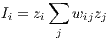
According to the demand perspective, tourism attractions are seen as ‘raw materials’ of this sector and are location-specific. As a result, tourism-dependent industries – beginning with accommodation and foodservices – locate themselves as near as possible to these attractions, which draw visitors (OECD 2008).
Illustrating this fact, the majority of accommodation companies are distributed in Romania’s mountain areas, Black Sea region, Delta of Danube and various cities (Figure 1). The most important localities are Bucuresti, Eforie, Costinesti, Brasov, Busteni, Constanta, Mangalia, Moeciu, Bran, Baile Felix, Predeal, Sibiu, Cluj-Napoca, Sinaia, Suceava, Iasi and Timisoara, many of them combining the natural and historic-cultural heritage attractions.
Sources: National Geographic, ESRI ArcGIS 2016 for topographic data; Romanian National Authority for
Tourism 2014 for thematic data
The top localities with the largest number of companies in the foodservice industry show the following ranking: Constanta, Cluj-Napoca, Arad, Mangalia, Bucharest, Brasov, Timisoara, Predeal, Sinaia. In this list there are large cities, mountain and seashore resorts. The distribution of all companies represented in the foodservice sector is presented in Figure 2.
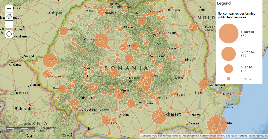
Sources: National Geographic, ESRI ArcGIS 2016 for topographic data; Romanian National Authority for
Tourism 2014 for thematic data
In addition to these two maps it is noteworthy to mention that there is a positive correlation between the distributions of accommodation and foodservice units and the areas with a higher urbanisation index, as shown by Figure 3, which presents a map of the urbanisation index.
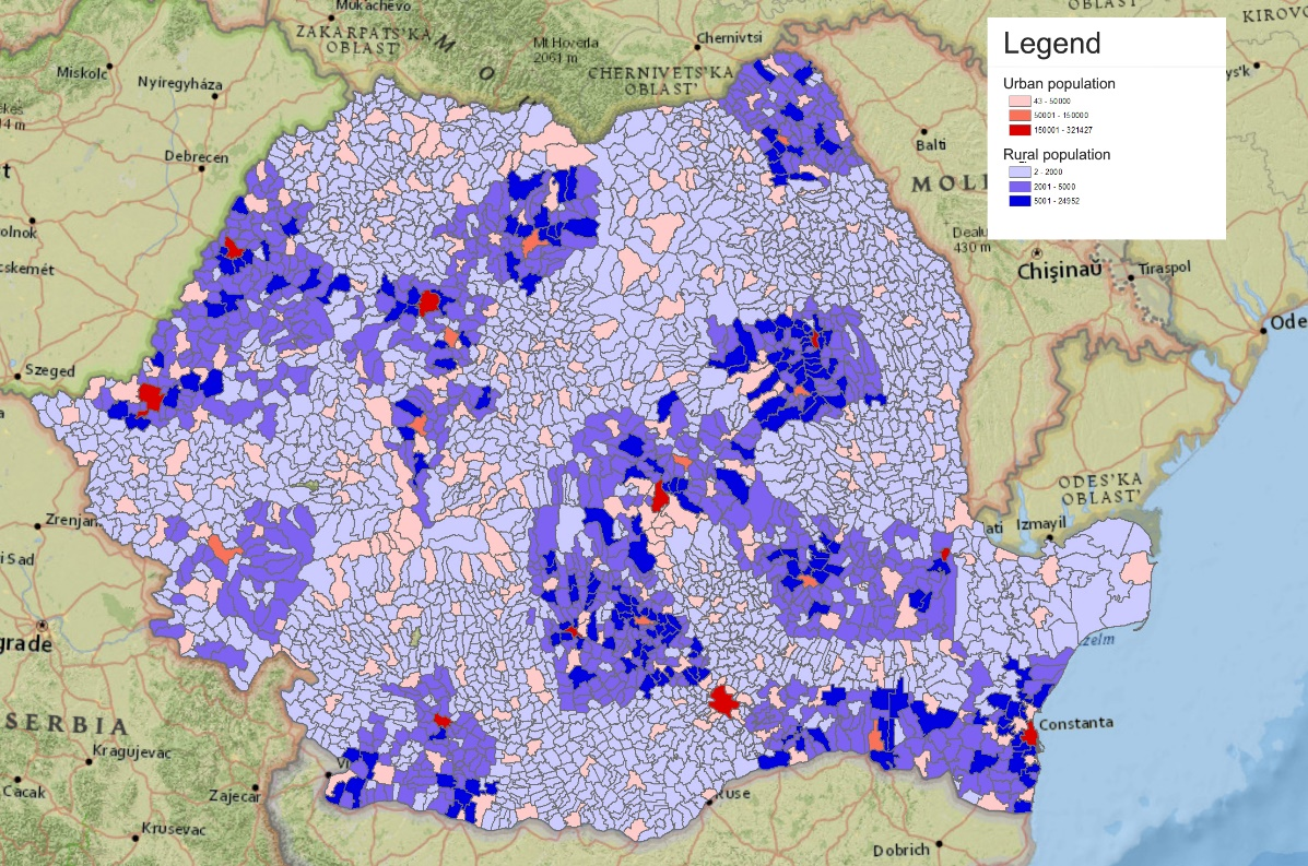
Source: ArcGIS 2016 for the administrative boundaries, National Institute of Statistics 2016 for thematic
data
3.2 Spatial Autocorrelation Analysis
3.2.1 Univariate spatial correlation
The map of locations that have a significant Moran index (for p-values below 0.05 and 0.01) corresponding to the “number of accommodation companies” variable is presented in Figure 4.
Sources: ArcGIS 2016 for the administrative boundaries, Romanian National Authority for Tourism 2014 for
thematic data
The significance map shows the locations with a significant Local Moran index, by using different shades of green depending on the p-value4 .
In the first category, for p < 0.05 there are 214 LAUs (light green) and in the second category, for p < 0.01 there are 774 LAUs (deep green). For the rest of LAUs, the local Moran index is not significant.
For the significant associations of LAUs in the case of the “number of accommodation companies” variable, the map in Figure 5 offers the interpretation of this univariate Local Moran, exploring the type of autocorrelation and the category of spatial association. For the considered variables, all 988 LAUs are included in positive autocorrelation agglomerations, two categories of spatial associations being distinguished: the first (in red), with 198 LAUs, indicates ‘high-high’ similarity based spatial clusters (agglomerations) (each LAU with a high value is surrounded by neighbours with high values too); the second (in blue), with 790 LAUs, indicates ‘low-low’ similarity based spatial associations, with a small number of accommodation units. This configuration is a confirmation of the first category incorporating the most important tourist areas in Romania (Black Sea, Delta of Danube, Prahova Valley, Bucovina, etc.), which indicates a ‘natural clusterisation’ as a response to the natural and, in some cases, historic and cultural environment advantages rather than the result of a clearly targeted tourism-support policy.
Sources: ArcGIS 2016 for the administrative boundaries, Romanian National Authority for Tourism 2014 for
thematic data
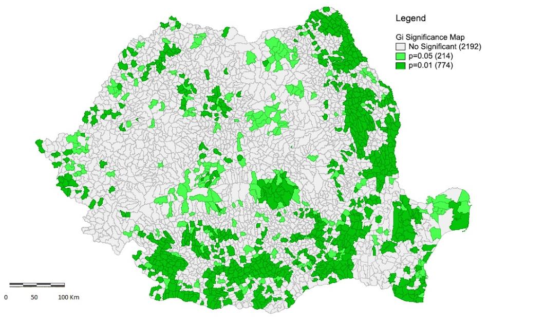
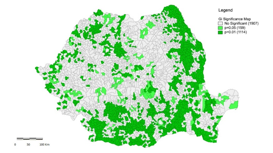
The same type of maps have been produced for the number of foodservice companies. The
significance map (Figure 6) indicates 159 LAUs for p < 0.05 and 1114 LAUs for p < 0.01.
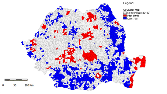
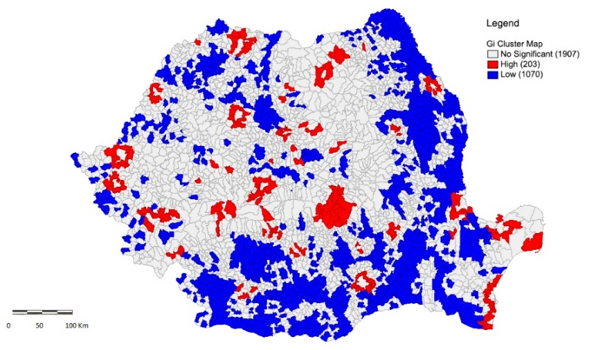
Subsequently, Figure 7 shows ‘high-high’ similarity based spatial agglomerations with 203
LAUs and ‘low-low’ similarity based spatial associations with 1070 LAUs. According to this
Gi cluster map, the largest agglomerations of foodservice companies are found in
Brasov, Bucharest, Constanta, Tulcea, Braila, Gala i, Arad, Timi
 , Re
, Re i
i a,
Caransebe
a,
Caransebe , Ia
, Ia i, Suceava, Câmpulung Moldovenesc, Cluj, Sibiu, Alba. Important tourist
attractions are located in all of these areas. For example, Constanta is the oldest
continuously inhabited city in Romania (since 600 BC) and the largest city on the
Romanian Black Sea coast, Tulcea is the gate to the Danube Delta, Suceava is Bucovina’s
historic capital, Brasov, Cluj, Sibiu are among the most attractive Transylvanian cities,
etc.
i, Suceava, Câmpulung Moldovenesc, Cluj, Sibiu, Alba. Important tourist
attractions are located in all of these areas. For example, Constanta is the oldest
continuously inhabited city in Romania (since 600 BC) and the largest city on the
Romanian Black Sea coast, Tulcea is the gate to the Danube Delta, Suceava is Bucovina’s
historic capital, Brasov, Cluj, Sibiu are among the most attractive Transylvanian cities,
etc.
Sources: ArcGIS 2016 for the administrative boundaries, Romanian National Authority for Tourism 2014 for
thematic data
Sources: ArcGIS 2016 for the administrative boundaries, Romanian National Authority for Tourism 2014 for
thematic data
3.2.2 Bivariate spatial correlation
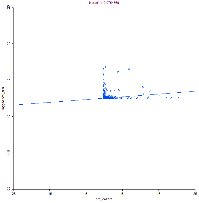
Moran’s scatterplot for spatial correlation between the number of accommodation companies and the number of foodservice companies is presented in Figure 8.
The value of Global Moran’s I is 0.07. This value is positive, suggesting a positive spatial autocorrelation between the number of accommodation companies and the number of foodservice companies, but very low. Furthermore, the Geary’s C has been also calculated. Its value is 0.7, confirming the positive spatial autocorrelation. Considering these results, one can conclude that the spatial autocorrelation exists in only some areas, mainly in the tourist areas. Nevertheless, the calculation and analysis of Local Moran’s I (LISA) is recommended in order to identify the geographic areas with local spatial associations in tourism infrastructure.
Sources: Romanian National Authority for Tourism 2014 for thematic data
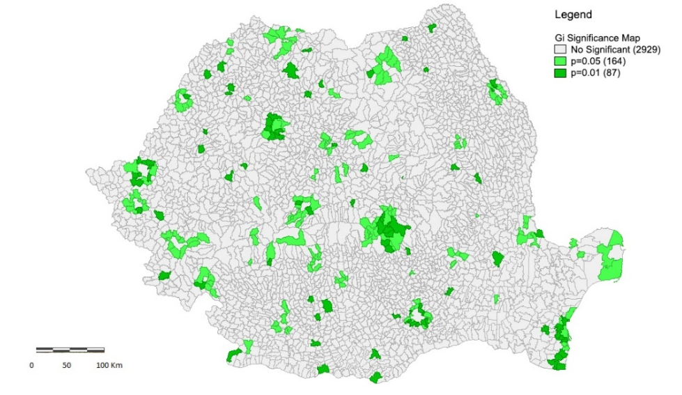
The map of locations with significant bivariate spatial correlation between the number of accommodation companies and the number of foodservice companies (significant bivariate Local Moran index), for p-values below 0.05 and 0.01 is presented in Figure 9. In the first category, for p < 0.05, 164 LAUs are included and in the second category, for p < 0.01 there are 87 LAUs. Large areas with significant bivariate Local Moran indices are inside the following counties: Brasov, Bucharest, Constanta Timis, Arad, Cluj, Maramures, Sibiu, Iasi, Bihor, Tulcea and Suceava, many of them including the most important tourist attractions in Romania.
Sources: ArcGIS 2016 for the administrative boundaries, Romanian National Authority for Tourism 2014 for
thematic data
The map with significant spatial associations of LAUs for the cross-correlation between the number of accommodation companies and the number of foodservice companies is presented in Figure 10. It reveals two classes (categories) of positive spatial correlations (‘high-high’ and ‘low-low’) and two classes of negative spatial correlation (‘high-low’ and ‘low-high’). Usually the spatial associations corresponding to positive correlations are named ‘spatial clusters’5 whereas those corresponding to negative correlations are associated with the ‘spatial outlier’ notion (Anselin et al. 2002).
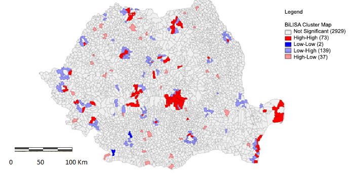
Sources: ArcGIS 2016 for the administrative boundaries, Romanian National Authority for Tourism 2014 for
thematic data
The four colour codes used for representing the four classes (categories) of significant associations of LAUs are as follows:
- dark red:
- for representing LAUs with a large number of accommodation companies surrounded by neighbouring LAUs with a large number of foodservice companies;
- dark blue:
- for representing LAUs with a small number of accommodation companies and surrounded by neighbouring LAUs with a small number of foodservice companies;
- pink:
- for LAUs with a large number of accommodation companies (‘high outlier in’), but surrounded by neighbouring LAUSs with a low number of foodservice companies (‘low neighbours in’);
- light blue:
- for LAUs where there is a small number of accommodation companies (‘low outlier in’), but surrounded by LAUs with a large number of foodservice companies (‘high neighbours in’).
Considering the frequency and the significance of each class of spatial association, two categories are of a particular interest for policy purposes, namely:
- 1.
- dark red (‘high-high’) spatial clusters, indicating the traditional, well-developed tourist areas such as the Black Sea area, Danube Delta, Prahova Valley (mountain tourism), Maramures (traditional village/rural and mountain tourism), Bucovina (traditional village/rural and ecumenical tourism), Valcea and Harghita counties (balnear and mountain tourism), Sibiu area (mountain, traditional village/rural and cultural tourism) and Cluj-Napoca area (cultural tourism). They can be considered functional tourist areas – interpreted as differentiated geographical areas characterised by “a concentration of uses, activities and visitation related to tourism”, which incorporates “clear references to varied elements of natural space – area, concentration, soil usage, visitation and frontiers” (Panosso Netto, Trigo 2015, p. 66, with reference to Haylar et al. 2008). In these areas investment support is necessary in order to boost their competitiveness not only in a national but also an international context via increased quality and diversification of the provided services. At the same time the policy-makers’ attention should be directed to actions able to develop working tourist clusters, with strong organisation of the inter-firm relations as well as advanced networks between all significant local actors.
- 2.
- light blue spatial associations (‘low-high’), where LAUs with relatively small number of accommodation units are surrounded by LAUs with a large number of foodservice units. This is the case in the metropolitan areas of the big cities (e.g. Bucharest, Constanta, Timisoara, Iasi, Cluj-Napoca, Galati, Oradea), where the interest in dining out in attractive natural areas is very high. In these areas the mixed restaurants prevail: they are visited by many locals and also draw important flows of tourists after the exploration of the tourist attractions specific to the urban environment (historic and art monuments, museums, exhibitions, etc.)6. In such cases efforts must be concentrated on providing good access infrastructure combined with rational land use in order to preserve the natural, green areas surrounding big cities.
In addition, considering the well-balanced distribution of natural and cultural-historic landscapes in Romania, adequate actions are recommended in order to create and promote new tourist destinations especially in regions that are lagging behind, where, so far, the map does not indicate significant spatial associations of LAUs in terms of number of accommodation and foodservice units. A particular case in this respect is represented by the pink spatial associations (‘high-low’), indicating LAUs with a relatively high number of accommodation units surrounded by LAUs with a small number of foodservice units. These associations are placed in less developed areas with good potential for future development of tourism, but which are insufficiently exploited so far. The low level of income of the inhabitants in these areas was not able to stimulate the growth of the foodservice sector – restaurants primarily visited by locals.
In a broader perspective, the Appendix presents simple descriptive statistics that illustrate the imbalances at county level between the existing tourism infrastructure (accommodation and foodservice segments) and the number of incoming tourists. For example, the ratio between the number of incoming tourists and accommodation companies acting in each county varies between 213.2 and 5689.8, indicating that in some geographical areas the existing accommodation infrastructure is poorly correlated with demand. Such findings should be considered for laying the foundations of more rational decisions with regard to the future distribution of funding (EU support included) for the support of tourism infrastructure development.
4 Concluding Remarks and Further Developments
Our inquiry into the spatial distribution of the tourism infrastructure in Romania – the accommodation and foodservice components – has revealed the main patterns in this respect, highlighted significant spatial cross-correlations between them and discussed their implications for the future development of tourism, thus responding to the research questions formulated in the paper introduction.
The performed analysis can be considered helpful from a theoretical point of view, based on its capability to improve methodologies for examining the relationships between companies participating in tourism activities and the landscape elements, for conceptualizing and identifying functional tourism areas. Furthermore, the performed investigation is helpful for practitioners too, as it provides useful information for selecting sites for new businesses in the tourism industry, as well as for policy-makers highlighting those tourist areas where additional support for their development could be beneficial.
The analysis has confirmed the working hypotheses with regard to the uneven territorial distribution of tourism infrastructure compared to the location of tourist attractions, the large number of spatial associations in the ‘low-high’ and ‘high-low’ classes suggesting significant differences between the geographical distribution of the accommodation and foodservice companies and the need for differentiated policies supporting tourism infrastructure, according to the specific necessities of the tourist areas.
However, this exploratory research should be seen as just a first step of a larger inquiry, able to offer a broader view on the spatial associations with relevant tourist activity. To this end, further investigation would envisage a wider range of indicators characterizing tourism development (e.g. number of beds in tourist accommodation units, number of accommodation units by quality class, number of arrivals, number of overnight stays, etc.), as well as indicators regarding the social-economic development level, the access to transportation infrastructure and so on. Also, the robustness of findings needs to be considered, so as to check whether the results are stable over time.
Another future direction of investigation points at the internal features of the ‘spatial clusters’ in the meaning derived from the interpretation of the univariate and bivariate Local Moran index: in other words, to what extent these significant spatial associations (and agglomerations of firms) exhibit the characteristics of tourist clusters, as clusters ‘á la Porter’, i.e. geographic concentrations of tourist resources and attractions, related infrastructure, equipment and service firms and other supporting sectors and administrative institutions with integrated and coordinated activities (Kirschner 2015). And, even if this paper cannot provide the empirical evidence necessary for establishing the stage of development, the simple existence of tourist clusters in the ‘dark red’ areas may also suggest the other side of the coin, namely competition relationships, which can be a source of increasing the quality of tourist services. Such relationships would also be interesting to explore.
In methodological terms, as mentioned by van Herwijnen et al. (2004), the success in applying GIS techniques for local or regional planning is closely related to the responses to requirements such as the meeting of scientific credibility standards (.i.e. very good links between GIS and spatial statistics, etc.) and the provision of customized products for scientific analysis. In such a context the local indicators of spatial association – local Moran index included – are seen as useful instruments for identifying local spatial clusters and for assessing the influence of a single location on the corresponding global statistics (Symanzik 2014). They can also be employed for highlighting influential points in a regression framework, representing a further direction of investigation for our research.
Acknowledgement
The exchange of ideas on the paper topic with our colleague, Professor Zizi Goschin, as well as the suggestions received from the participants in the special session dedicated to Manfred Fischer at the 55th ERSA Congress in Lisbon, 2015 and, subsequently, from the paper reviewers are gratefully acknowledged.
References
Anselin L (1995) Local indicators of spatial association – LISA. Geographical Analysis 27[2]: 93–115. CrossRef.
Anselin L, Syabri I, Smirnov O (2002) Visualising multivariate spatial correlation with dynamically linked windows. In Anselin L, Rey S (eds.), New tools for spatial data analysis: proceedings of the specialist meeting, Center for Spatially Integrated Social Science (CSISS), University of California, Santa Barbara, CD-ROM
Brown G (2006) Mapping landscape values and development preferences: A method for tourism and residential development planning. International Journal of Tourism Research 8[2]: 101–113. CrossRef.
Chancellor C, Cole S (2008) Using geographic information system to visualize travel patterns and market research data. Journal of Travel & Tourism Marketing 25[3]: 341–54
Cheng T, Haworth J, Anbaroglu B (2014) Spatiotemporal data mining. In: Fischer MM, Nijkamp P (eds), Handbook of Regional Science. Springer, Berlin Heidelberg, 1173–1194. CrossRef.
Chung W, Kalnins A (2001) Agglomeration effects and performance: A test of Texas lodging industry. Strategic Management Journal 22: 969–988. CrossRef.
Constantin DL, Mitrut C (2009) Cultural tourism, sustainability and regional development: Experiences from Romania. In: Fusco-Girard L, Nijkamp P (eds), Cultural Tourism and Sustainable Local Development. Ashgate, Farnham, 149–166
de Dominicis L, Arbia GL, Groot H (2007) Spatial distribution of economic activities in local labour market areas: The case of Italy. Tinbergen institute discussion paper, 07-094/3, Amsterdam-Rotterdam
Dubé J, Legros D (2014) Spatial Econometrics Using Microdata. John Wiley & Sons, London. CrossRef.
Feng R, Morrison AM (2002) GIS applications in tourism and hospitality marketing: A case in Brown County, Indiana. Anatolia: An International Journal of Tourism and Hospitality Research 13[2]: 127–143
Gaughan AE, Binford MW, Southworth J (2009) Tourism, forest conversion and land transformations in the Angkor basin, Cambodia. Applied Geography 29[2]: 212–223. CrossRef.
Goschin Z (2015) Evolution of wage and unemployment gaps in the context of economic crisis: A spatial perspective. Romanian Journal of Regional Science 9[1]: 17–33
Griffith DA (2003) Spatial Autocorrelation and Spatial Filtering: Gaining Understanding Through Theory and Scientific Visualization. Springer, Berlin Heidelberg
Griffith DA, Chun Y (2014) Spatial autocorrelation and spatial filtering. In: Fischer MM, Nijkamp P (eds), Handbook of Regional Science. Springer, Berlin Heidelberg, 1477–1508. CrossRef.
Haining R (2014) Spatial data and statistical methods: A chronological overview. In: Fischer MM, Nijkamp P (eds), Handbook of Regional Science. Springer, Berlin Heidelberg, 1277–1294. CrossRef.
Haylar B, Griffin T, Edwards D (2008) City Spaces – Tourist Places. Elsevier, London. CrossRef.
Kalnins A, Chung W (2004) Resource-seeking agglomeration: A study of market entry in the lodging industry. Strategic Management Journal 25: 689–699. CrossRef.
Kang S, Kim J, Nicholls S (2014) National tourism policy and spatial patterns of domestic tourism in South Korea. Journal of Travel Research 53[6]: 791–804. CrossRef.
Kirschner T (2015) Tourism clusters – a model for the development of innovative tourist products. Carpathian tourist cluster, available at www.tourism-cluster-romania.com
Lau G, McKercher B (2006) Understanding tourist movement patterns in a destination: A GIS approach. Tourism and Hospitality Research 7[1]: 39–49. CrossRef.
Li M, Fang L, Huang X, Goh C (2014) A spatial-temporal analysis of hotels in urban tourism destination. International Journal of Hospitality Management 45: 34–43
Marco-Lajara B, Claver-Cortes E, Ubeda-Garcia M, Zaragoza-Saez PC (2016) Do hotels benefit from agglomeration? Journal of Tourism and Hospitality 5[1]: 1–5
OECD – Organisation for Economic Co-operation and Development (2008) Tourism in OECD countries 2008: Trends and policies. Organisation for Economic Co-operation and Development, February
Panosso Netto A, Trigo LGG (2015) Tourism in Latin America: Cases of Success. Springer, Berlin Heidelberg
Pearce DG (1995) Tourism Today: A Geographical Analysis (2nd ed.). Longman, Harlow
Poslad S, Laamanen H, Malaka R, Nick A, Buckle P, Zipl A (2001) Crumpet: creation of user-friendly mobile services personalised for tourism. Paper presented at the 3G mobile communication technologies, 2001 – second international conference, available at: http://195.130.87.21:8080/dspace/bitstream/123456789/576/1/Crumpet creation of user-friendly mobile services personalised for tourism.pdf
Salo A, Garriga A, Rigall-I-Torrent R, Vila M, Fluvia M (2014) Do implicit prices for hotels and second homes show differences in tourists’ valuation for public attributes for each type of accommodation facility? International Journal of Hospitality Management 36[1]: 120–129. CrossRef.
Seul KL (2015) Quality differentiation and conditional spatial price competition among hotels. Tourism Management 46: 114–122. CrossRef.
Shoval N, McKercher B, Ng E, Birenboim A (2011) Hotel location and tourist activity in cities. Annals of Tourism Research 38[4]: 1594–1612. CrossRef.
Symanzik J (2014) Exploratory spatial data analysis. In: Fischer MM, Nijkamp P (eds), Handbook of Regional Science. Springer, Berlin Heidelberg, 1295–1130. CrossRef.
Terhorst P, Erkus-Öztürk H (2016) Beyond fordism and flexible specialization in Antalya’s mass-tourism economy. In: Egresi I (ed), Alternative Tourism in Turkey: Role, Potential Development and Sustainability. Springer, Berlin. CrossRef.
van Herwijnen M, Hanssen R, Nijkamp P (2004) A multi-criteria decision support model and geographic information system for sustainable development planning of the Greek Islands. In: Nijkamp P (ed), Environmental Economics and Evaluation. Edward Elgar, Cheltenham
WEF – World Economic Forum (2013) The travel and tourism competitiveness report 2013: Reducing barriers to economic growth and job creation. World Economic Forum, Geneva, available at http://www.weforum.org/ttcr
Williams AM, Shaw G (1995) Tourism and regional development polarization and new forms of production in the United Kingdom. Tijdschrift voor Economische en Sociale Geografie 86[1]: 50–63. CrossRef.
Yang Y, Hao L, Rob L (2014) Theoretical, empirical and operational models in hotel location research. International Journal of Hospitality Management 36: 209–220. CrossRef.
Zhang HQ, Guillet BD, Gao W (2012) What determines multinational hotel groups’ locational investment choice in China? International Journal of Hospitality Management 31[2]: 350–359. CrossRef.
Zhang Y, Xu JH, Zhuang PJ (2011) The spatial relationship of tourist distribution in Chinese cities. Tourism Geographies: An International Journal of Tourism Space, Place and Environment 13[1]: 75–90
Appendix: Descriptive statistics of tourism infrastructure available in Romania at county level in 2015
| Ratio No. | ||||||
| of | ||||||
| incoming | ||||||
| No. of | No. of | RANK | tourists/ | |||
| Food | Accommo- | Accommo- | No. of | RANK | accommo- | |
| Services | dation | dation | Incoming | Incoming | dation | |
| Companies | Companies | Companies | Tourists | Tourists | companies | |
| ALBA | 86 | 233 | 18 | 154210 | 19 | 661.8 |
| ARAD | 413 | 166 | 21 | 214826 | 13 | 1294.1
|
| ARGES | 143 | 286 | 15 | 195200 | 14 | 682.5 |
| BACAU | 112 | 173 | 20 | 124517 | 22 | 719.8
|
| BIHOR | 155 | 330 | 9 | 344059 | 8 | 1042.6 |
| BISTRITA NASAUD | 56 | 76 | 29 | 80293 | 28 | 1056.5
|
| BOTOSANI | 17 | 28 | 39 | 37670 | 38 | 1345.4 |
| BRAILA | 41 | 44 | 35 | 71417 | 31 | 1623.1
|
| BRASOV | 586 | 1139 | 2 | 997601 | 3 | 875.9 |
| BUCURESTI | 308 | 303 | 13 | 1723999 | 1 | 5689.8
|
| BUZAU | 82 | 112 | 25 | 68295 | 33 | 609.8 |
| CALARASI | 13 | 22 | 41 | 17809 | 41 | 809.5
|
| CARAS SEVERIN | 223 | 246 | 17 | 171626 | 16 | 697.7 |
| CLUJ | 695 | 355 | 7 | 428812 | 7 | 1207.9
|
| CONSTANTA | 1555 | 1263 | 1 | 1021475 | 2 | 808.8 |
| COVASNA | 59 | 147 | 23 | 88800 | 26 | 604.1
|
| DAMBOVITA | 66 | 87 | 26 | 89548 | 25 | 1029.3 |
| DOLJ | 63 | 75 | 31 | 102486 | 23 | 1366.5
|
| GALATI | 75 | 48 | 34 | 74416 | 30 | 1550.3 |
| GIURGIU | 9 | 33 | 37 | 24860 | 40 | 753,3
|
| GORJ | 58 | 152 | 22 | 78418 | 29 | 515,9
|
| HARGHITA | 147 | 462 | 5 | 157659 | 17 | 341,3
|
| HUNEDOARA | 151 | 300 | 14 | 151060 | 20 | 503.5
|
| IALOMITA | 36 | 27 | 40 | 44863 | 34 | 1661.6
|
| IASI | 106 | 115 | 24 | 246470 | 12 | 2143.2
|
| ILFOV | 48 | 75 | 32 | 126858 | 21 | 1691.4
|
| MARAMURES | 137 | 341 | 8 | 154633 | 18 | 453.5
|
| MEHEDINTI | 46 | 79 | 28 | 81003 | 27 | 1025.4
|
| MURES | 216 | 327 | 10 | 495481 | 4 | 1515.2
|
| NEAMT | 130 | 277 | 16 | 182384 | 15 | 658.4
|
| OLT | 28 | 35 | 36 | 33343 | 39 | 952.7
|
| PRAHOVA | 266 | 572 | 3 | 467158 | 5 | 816.7
|
| SALAJ | 28 | 52 | 33 | 37962 | 36 | 730
|
| SATU MARE | 40 | 82 | 27 | 94908 | 24 | 1157.4
|
| SIBIU | 147 | 447 | 6 | 438611 | 6 | 981.2
|
| SUCEAVA | 262 | 506 | 4 | 310548 | 10 | 613.7
|
| TELEORMAN | 5 | 18 | 42 | 13214 | 42 | 734.1
|
| TIMIS | 199 | 229 | 19 | 338238 | 9 | 1477
|
| TULCEA | 110 | 324 | 11 | 69076 | 32 | 213.2
|
| VALCEA | 181 | 316 | 12 | 286892 | 11 | 907.9
|
| VASLUI | 19 | 29 | 38 | 37886 | 37 | 1306.4
|
| VRANCEA | 40 | 76 | 30 | 43290 | 35 | 569.6
|
| Total | 7157 | 10007 | 9921874 | |||
| Mean | 170.4 | 238.3 | 236235.1 | 536.8 | ||
| Median | 96.0 | 159.0 | 125687.5 | 515.9 | ||
| standard deviation | 262.8 | 264.1 | 325282.6 | 206.8 | ||